
Multi-objective Bayesian optimization with
reference point – sequential and parallel versions
David Gaudrie
1,2
, Rodolphe Le Riche
1
, Victor Picheny
3
,
Benoˆıt Enaux
2
, Vincent Herbert
2
1
CNRS LIMOS at Mines Saint-Etienne, France
2
PSA
3
Prowler.io
20 March 2019
GDR Mascot-Num annual conference
IFPEN, Rueil-Malmaison, France
R. Le Riche et al. (CNRS EMSE) Sequential and parallel R/C-mEI 1/55 March 2019 1 / 55

Goal: multi-objective optimization (1)
In general there are many (even an infinite number of) trade-off
solutions to
min
x∈X ⊂R
d
(f
1
(x), . . . , f
m
(x))
called the Pareto set (in X ) or front (in Y).
It is composed of Non-Dominated points,
{x ∈ X : @x
0
6= x ∈ X , ∀i f
i
(x
0
) ≤ f
i
(x) & ∃ j f
j
(x
0
) < f
j
(x)}.
C is dominated,
A and B non-
dominated
Notation:
A ≺ C, B ≺ C
R. Le Riche et al. (CNRS EMSE) Sequential and parallel R/C-mEI 2/55 March 2019 2 / 55


Curse of dimensionality: number of variables
At a given budget, optimization performance degrades with the
number of variables:
d = 3 d = 22
(optimization algorithm: EHI – Emmerich et al. [3] – with GPareto – Binois and Picheny [1])
R. Le Riche et al. (CNRS EMSE) Sequential and parallel R/C-mEI 4/55 March 2019 4 / 55

Curse of dimensionality: number of objectives (1)
At a given budget, optimization performance degrades with the
number of objectives:
(optimization algorithm: EHI – Emmerich et al. [3] – with GPareto – Binois and Picheny [1])
R. Le Riche et al. (CNRS EMSE) Sequential and parallel R/C-mEI 5/55 March 2019 5 / 55

Curse of dimensionality: number of objectives (2)
As the number of objectives increases, a larger part of X becomes Pareto optimal:
m = 2 m = 3
Ex: sphere functions centered on C1, C2, C3. Pareto sets (in red) are all convex
combinations of the C’s. Blue triangles: points sampled by MO Bayesian
algorithm (GPareto). With 4 objectives at the corners of X , every point could be
a Pareto solution. As the Pareto set becomes larger, the optimization algorithm
degenerates in a space filling algorithm. Give up the utopian search for all of the
Pareto set.
R. Le Riche et al. (CNRS EMSE) Sequential and parallel R/C-mEI 6/55 March 2019 6 / 55

Restricting ambitions in MOO of costly functions
Metamodels of costly functions does not solve everything: they still need
to be learned. Recently, we have explored ways to proportionate ambitions
to search budget (about 100 functions evaluations):
Today’s talk: how to focus on specific regions of the Pareto
front. The R-mEI algorithm explained step by step:
1
Finding one Pareto optimal point
2
Widening the search
3
A q-points batch version
Details and proofs in [6, 7].
See also: variable dimension reduction:
variables selection for optimization (m = 1). Work with Adrien
Spagnol and S´ebastien Da Veiga, Safran Tech, cf. [16].
problem reformulation (eigenshapes), cf. other presentation by
David Gaudrie here.
R. Le Riche et al. (CNRS EMSE) Sequential and parallel R/C-mEI 7/55 March 2019 7 / 55

MOO: related work (1)
Evolutionary Multi-objective Optimization (EMO): a field in
itself (10 EMO international conferences, Deb’s book [12]),
expensive without model of the function.
Model-based multi-objective optimization:
gradient on Gaussian Process (GP) mean (Zerbinati et al. [19]),
the family of Bayesian MOO (EHI, SMS, SUR, EMI – GPareto
[1], Wagner et al. [17] –), constrained EHI (Feliot et al. [4]).
They target the entire front, cheaper than EMO but still
expensive for us (curse of criteria dimensionality, see earlier).
R. Le Riche et al. (CNRS EMSE) Sequential and parallel R/C-mEI 8/55 March 2019 8 / 55

MOO: related work (2)
User preference: scalarize the
MOO by minimizing a
distance to a user given goal,
min
x∈X
dist(f(x), goal)
(Miettinen [15]). But choice
of the metric, choice of the
goal.
f
1
f
2
L
∞
metric
L
1
metric
L
2
metric
goal
f(X)
User preference in Bayesian optimization: weighted EHI (Feliot et
al. [5]), truncated EHI (Yang et al. [18]). But: need to specify
the weight or the truncation region.
⇒ we now propose a Bayesian MOO with or without user
preference (reference point and its default), R/C-mEI.
R. Le Riche et al. (CNRS EMSE) Sequential and parallel R/C-mEI 9/55 March 2019 9 / 55


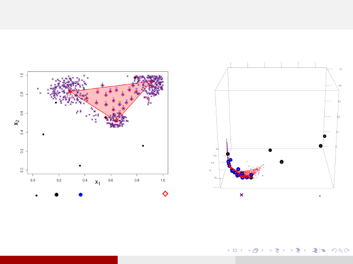
Simulations points for the Pareto front (1)
The choice of the x’s where the simulations are performed matters.
Below, blue points are random, red points selected proportionally to
their probability of being non dominated by the empirical front
c
P
Y
:
(d = 22)
R. Le Riche et al. (CNRS EMSE) Sequential and parallel R/C-mEI 12/55 March 2019 12 / 55

Simulations points for the Pareto front (2)
Choose x’s with a probability proportional to P
c
P
Y
Y(x)
.
In the quadratic case, d = 2, m = 3, after 20 iterations
DoE & & , Non Dominated , selected point , sampled Y ND
Simulation points are uniformly distributed near the Pareto set.
R. Le Riche et al. (CNRS EMSE) Sequential and parallel R/C-mEI 13/55 March 2019 13 / 55

Bayesian multi-objective optimization (1)
Where to put the next point, x
n+1
, where to call the costly f? At the
point that maximizes, on the average of the Y(x) samples, the
Hypervolume Improvement (over the empirical Pareto front
c
P
Y
):
H(A; R) =
[
y∈A
Z
yzR
dz
I
H
(f; R) = H(
c
P
Y
∪ {f}; R) − H(
c
P
Y
; R)
EHI(x; R) = E (I
H
(Y(x); R))
EHI favors Y(x) dominating the
empirical Pareto front and far from
already observed f(x
i
)s.
Notice: the omnipresence of R;
∀R
c
P
Y
, EHI generalizes the EI
criterion of EGO (Jones [10]).
EHI implementation from [14]
R. Le Riche et al. (CNRS EMSE) Sequential and parallel R/C-mEI 14/55 March 2019 14 / 55

Bayesian multi-objective optimization (2)
Algorithm 1 Multi-objective EHI Bayesian optimizer
Require: DoE = {(x
1
, f(x
1
)), . . . , (x
n
, f(x
n
))}, R, n
max
1: while n < n
max
do
2: Build m independent GPs, Y() = (Y
1
(), . . . , Y
m
()), from cur-
rent DoE
3: Find next iterate by solving x
n+1
= arg max
x∈X
EHI(x; R)
{internal optimization problem, no call to f()}
4: Calculate f(x
n+1
)
5: n ← n + 1
6: end while
R. Le Riche et al. (CNRS EMSE) Sequential and parallel R/C-mEI 15/55 March 2019 15 / 55

Targeting improvement regions with EHI
To find the entire Pareto front, R must be dominated by the Nadir
point, N: R1 is the default in the litterature.
But the entire Pareto front
is i) too large to be de-
scribed ii) not interesting
in general (e.g., extreme
solutions).
⇒ move R and control the
improvement region,
I
R
:
= {y ∈ Y : y R}
(keeps the Pareto rank for
non comparable functions)
R1
N
I
R. Le Riche et al. (CNRS EMSE) Sequential and parallel R/C-mEI 16/55 March 2019 16 / 55


mEI, a computationally efficient proxy to EHI
Once R is freed from
c
P
Y
, a new acquisition criterion is possible.
Definition:
mEI(x; R)
:
=
Q
m
j=1
EI
j
(x; R
j
)
Y ’s indep.
= E
Q
m
j=1
max(0 , R
j
− Y
j
(x))
Property:
If
c
P
Y
R, EHI(·; R) = mEI(·; R).
mEI(x; R) is analytical in m
i
(x) and C
i
(x, x), computationally much more efficient
than EHI which involves Monte Carlo simulations when m > 2 (ms vs min).
R. Le Riche et al. (CNRS EMSE) Sequential and parallel R/C-mEI 18/55 March 2019 18 / 55


Reference point updating: principle
b
R too ambitious (e.g.,
near Ideal): the algorithm
degenerates into a space
filling (variance driven).
b
R easy to reach: favors
already known high
achievers.
⇒
b
R near the Empirical Pareto front as
the right amount of ambitions (explo-
ration vs intensification).
●
●
●●
●
●
●
●
●
●
●
●
●
●
●
●
●
●
●
●
●
●
●
●
●
●
●
●
●
●
●
●
●
●
●
●
●
●
●
●
●
●
●
●
●
●
●
●
●
●
●
●
●
●
●
●
●
●
●
●
●
●
●
●
●
●
●
●
●
●
●
●
●
●
●
●
●
●
●
●
●
●
●
●
●
●
●
●
●
●
●
●
●
●
●
●
●
●
●
●
●
●
●
●
●
●
●
●
●
●
●
●
●
●
●
●
●
●
●
●
●
●
●
●
●
●
●
●
●
●
●
●
●
●
●
●
●
●
●
●
●
●
●
●
●
●
●
●
●
●
●
●
●
●
●
●
●
●
●
●
●
●
●
●
●
●
●
●
●
●
●
●
●
●
●
●
●
●
●
●
●
●
●
●
●
●
●
●
●
●
●
●
●
●
●
●
●
●
●
●
●
●
●
●
●
●
●
●
●
●
●
●
●
●
●
●
●
●
●
●
●
●
●
●
●
●
●
●
●
●
●
●
●
●
●
●
●
●
●
●
●
●
●
●
●
●
●
●
●
●
●
●
●
●
●
●
●
●
●
●
●
●
●
●
●
●
●
●
●
●
●
●
●
●
●
●
●
●
●
●
●
●
●
●
●
●
●
●
●
●
●
●
●
●
●
●
●
●
●
●
●
●
●
●
●
●
●
●
●
●
●
●
●
●
●
●
●
●
●
●
●
●
●
●
●
●
●
●
●
●
●
●
●
●
●
●
●
●
●
●
●
●
●
●
●
●
●
●
●
●
●
●
●
●
●
●
●
●
●
●
●
●
●
●
●
●
●
●
●
●
●
●
●
●
●
●
●
●
●
●
●
●
●
●
●
●
●
●
●
●
●
●
●
●
●
●
●
●
●
●
●
●
●
●
●
●
●
●
●
●
●
●
●
●
●
●
●
●
●
●
●
●
●
●
●
●
●
●
●
●
●
●
●
●
●
●
●
●
●
●
●
●
●
●
●
●
●
●
●
●
●
●
●
●
●
●
●
●
●
●
●
●
●
●
●
●
●
●
●
●
●
●
●
●
●
●
●
●
●
●
●
●
●
●
●
●
●
●
●
●
●
●
●
●
●
●
●
●
●
●
●
●
●
●
●
●
●
●
●
●
●
●
●
●
●
●
●
●
●
●
●
●
●
●
●
●
●
●
●
●
●
●
●
●
●
●
●
●
●
●
●
●
●
●
●
●
●
●
●
●
●
●
●
●
●
●
●
●
●
●
●
●
●
●
●
●
●
●
●
●
●
●
●
●
●
●
●
●
●
●
●
●
●
●
●
●
●
●
●
●
●
●
●
●
●
●
●
●
●
●
●
●
●
●
●
●
●
●
●
●
●
●
●
●
●
●
●
●
●
●
●
●
●
●
●
●
●
●
●
●
●
●
●
●
●
●
●
●
●
●
●
●
●
●
●
●
●
●
●
●
●
●
●
●
●
●
●
●
●
●
●
●
●
●
●
●
●
●
●
●
●
●
●
●
●
●
●
●
●
●
●
●
●
●
●
●
●
●
●
●
●
●
●
●
●
●
●
●
●
●
●
●
●
●
●
●
●
●
●
●
●
●
●
●
●
●
●
●
●
●
●
●
●
●
●
●
●
●
●
●
●
●
●
●
●
●
●
●
●
●
●
●
●
●
●
●
●
●
●
●
●
●
●
●
●
●
●
●
●
●
●
●
●
●
●
●
●
●
●
●
●
●
●
●
●
●
●
●
●
●
●
●
●
●
●
●
●
●
●
●
●
●
●
●
●
●
●
●
●
●
●
●
●
●
●
●
●
●
●
●
●
●
●
●
●
●
●
●
●
●
●
●
●
●
●
●
●
●
●
●
●
●
●
●
●
●
●
●
●
●
●
●
●
●
●
●
●
●
●
●
●
●
●
●
●
●
●
●
●
●
●
●
●
●
●
●
●
●
●
●
●
●
●
●
●
●
●
●
●
●
●
●
●
●
●
●
●
●
●
●
●
●
●
●
●
●
●
●
●
●
●
●
●
●
●
●
●
●
●
●
●
●
●
●
●
●
●
●
●
●
●
●
●
●
●
●
●
●
●
●
●
●
●
●
●
●
●
●
●
●
●
●
●
●
●
●
●
●
●
●
●
●
●
●
●
●
●
●
●
●
●
●
●
●
●
●
●
●
●
●
●
●
●
●
●
●
●
●
●
●
●
●
●
●
●
●
●
●
●
●
●
●
●
●
●
●
●
●
●
●
−2.5 −2.0 −1.5 −1.0 −0.5 0.0 0.5 1.0
−1.5 −1.0 −0.5 0.0
f
1
f
2
●
●
●
Observed values
Empirical Pareto front
User supplied reference point
Estimated Ideal point
Readjusted reference point
●
●
●
●
●
●
●
●
●
●
●
●
●
●
●
●
I
R
R
No user preference (R)? Default with the Pareto front center (next).
R. Le Riche et al. (CNRS EMSE) Sequential and parallel R/C-mEI 20/55 March 2019 20 / 55

The Pareto front center
Which point should be targeted through R? By default, the point
where objectives are “balanced”.
Definition: The center C is the point of the Ideal-Nadir line the
closest in Euclidean distance to the Pareto front.
R. Le Riche et al. (CNRS EMSE) Sequential and parallel R/C-mEI 21/55 March 2019 21 / 55

Properties of the Pareto front center
The Pareto front center is equivalent, in game theory, to the
Kalai-Smordinsky solution with a disagreement point at the
Nadir [11].
The Pareto front center is invariant w.r.t. a linear scaling of the
objectives either when the Pareto front intersects the Ideal-Nadir
line, or when m = 2 (not true in general though).
The Pareto front center is stable w.r.t. perturbations in Ideal
and Nadir: k∆Ck
2
< k∆Nk
2
and k∆Ck
2
< k∆Ik
2
.
R. Le Riche et al. (CNRS EMSE) Sequential and parallel R/C-mEI 22/55 March 2019 22 / 55

Estimating the Pareto front center
Crude estimators:
b
I = ( min
y∈DoE
(y
1
), . . . , min
y∈DoE
(y
m
)),
b
N = (max
y∈
c
P
Y
(y
1
), . . . , max
y∈
c
P
Y
(y
m
)),
but they may be misleading early in the search. Take advantage of
the GPs uncertainties ⇒ estimate them from Pareto front simulations
(at carefully selected x’s, see next slides) and take their median.
R. Le Riche et al. (CNRS EMSE) Sequential and parallel R/C-mEI 23/55 March 2019 23 / 55

Simulation points for the Ideal and the Nadir (1)
(For the Pareto front, choose x’s with a probability proportional to
P
c
P
Y
Y(x)
.) ← see earlier
For the Ideal, choose x’s with a probability proportional to
P
Y
i
(x) ≤ min
j
f
j
i
, j = 1, n, i = 1, m (analytical).
For the Nadir, choose x’s with a probability proportional to
P
Y
i
(x) >
b
N
i
, Y(x) non dominated
+ P
Y(x) arg
b
N
i
, i = 1, m
More details in [6]
R. Le Riche et al. (CNRS EMSE) Sequential and parallel R/C-mEI 24/55 March 2019 24 / 55
Simulation points for the Ideal and the Nadir (2)
In the quadratic case, d = 2, m = 3, after 20 iterations
DoE & & , Non Dominated , selected point , sampled Y ND
Simulation points are grouped around the centers which make the Ideal and
Nadir.
R. Le Riche et al. (CNRS EMSE) Sequential and parallel R/C-mEI 25/55 March 2019 25 / 55

First phase of R estimations
Require: DoE =
{(x
1
, f(x
1
)), . . . , (x
n
, f(x
n
))},
n
max
1: Build the m independent
GPs;
2: repeat
3: if no R then
4: estimate Nadir
b
N;
R ←
b
N;
5: end if
6: estimate Ideal
b
I;
7:
b
R ← Project on
b
IR the
closest point of
c
P
Y
to
b
IR;
8: x
n+1
= arg max
x∈X
mEI(x;
b
R);
9: evaluate f(x
n+1
) and
update the GPs;
10: n ← n+1;
11: until n > n
max
Often
b
R is at the true Pareto front before the end. Cannot be further
improved. Waste of computation.
R. Le Riche et al. (CNRS EMSE) Sequential and parallel R/C-mEI 26/55 March 2019 26 / 55

Example of convergence to one Pareto-optimal
point
−2.5 −2.0 −1.5 −1.0 −0.5 0.0 0.5 1.0
−1.5 −1.0 −0.5 0.0
f
1
f
2
I
R
Pareto Front
Provided reference point
Reference points used by mEI
Last reference point used by mEI
Need a stopping criterion.
R. Le Riche et al. (CNRS EMSE) Sequential and parallel R/C-mEI 27/55 March 2019 27 / 55

Uncertainty in center location (1)
Need a stopping criterion. mEI and EHI are too unstable: depend on
f
i
’s scales and R.
Define the domination probability,
p(y)
:
= P (∃x ∈ X : Y(x) y)
Estimation: simulate n
sim
Pareto fronts (at well-chosen x’s),
f
P
Y
(i)
,
and
d
p(y) =
1
n
sim
n
sim
X
i=1
(
f
P
Y
(i)
y)
R. Le Riche et al. (CNRS EMSE) Sequential and parallel R/C-mEI 28/55 March 2019 28 / 55

Uncertainty in center location (2)
If
d
p(y) is near 1 or 0, we are quite sure that y is dominated or not.
The uncertainty is p(y)(1 − p(y)), the variance of the Bernouilli
variable D(y) = (P
Y()
y).
Define the uncertainty in
center location as
U(
b
L) :=
1
|
b
L|
Z
b
L
p(y)(1 − p(y))dy .
(d = 8)
R. Le Riche et al. (CNRS EMSE) Sequential and parallel R/C-mEI 29/55 March 2019 29 / 55

Finding one Pareto-optimal point
Algorithm 2 First phase of the R/C-mEI algorithm
Require: DoE = {(x
1
, f(x
1
)), . . . , (x
n
, f(x
n
))}, ε
1
, n
max
1: Build the m independent GPs;
2: repeat
3: estimate
b
R (i.e.,
b
I, and
b
N if no user reference);
4: x
n+1
= arg max
x∈X
mEI(x;
b
R);
5: evaluate f(x
n+1
) and update the GPs;
6: compute U(
b
IR);
7: n ← n+1;
8: until U(
b
L) ≤ ε
1
or n > n
max
(If no R, R defaults to
b
N and
b
R is
b
C)
R. Le Riche et al. (CNRS EMSE) Sequential and parallel R/C-mEI 30/55 March 2019 30 / 55


Remaining budget: second phase
What if convergence to the Pareto front occurs before n
max
?
⇒ widen the search around the last
b
R (or
b
C) by moving
b
R along
b
IR
away from the Ideal by a distance that is compatible with the
remaining budget, n
max
− n.
R. Le Riche et al. (CNRS EMSE) Sequential and parallel R/C-mEI 33/55 March 2019 33 / 55

Optimal final search region
For a given
b
R, anticipate the future space filling of the algorithm
by virtual iterates (Kriging Believer, [8]) ⇒ Y
KB
(x) built from
{(x
1
, f(x
1
)), . . . , (x
n
, f(x
n
))}
S
{(x
n+1
, µ(x
n+1
)), . . . , (x
n
max
, µ(x
n
max
))}
Measure the remaining uncertainty in Pareto domination
U(
b
R, Y) :=
1
Vol(
b
I,
b
R)
Z
b
Iy
b
R
p(y)(1 − p(y))dy .
Second phase optimal reference point defined through
R
∗
= arg max
b
R∈
b
IR
k
b
R −
b
Ik such that U(
b
R; Y
KB
) ≤ ε
2
(1)
by enumeration.
R. Le Riche et al. (CNRS EMSE) Sequential and parallel R/C-mEI 34/55 March 2019 34 / 55

Optimal final search region: illustration
The remaining uncertainty in Pareto domination can be seen by the sampled
fronts roaming (in grey). It is small enough on the left, too large on the right.
R
∗
is in blue. d = 8.
R. Le Riche et al. (CNRS EMSE) Sequential and parallel R/C-mEI 35/55 March 2019 35 / 55

Budgeted and Targeted MO Bayesian Optimization
Algorithm 3 The R-mEI algorithm
Require: DoE = {(x
1
, f(x
1
)), . . . , (x
n
, f(x
n
))}, ε
1
, ε
2
, n
max
1: Build the m independent GPs;
2: repeat
3: estimate
b
R (i.e.,
b
I, and
b
N if no user reference);
4: x
n+1
= arg max
x∈X
mEI(x;
b
R);
5: evaluate f(x
n+1
) and update the GPs;
6: compute U(
b
IR);
7: n ← n+1;
8: until U(
b
IR) ≤ ε
1
or n > n
max
9: if n < n
max
then
10: Calculate R
∗
solution of Eq. (1); # needs ε
2
11: end if
12: while n < n
max
do
13: x
n+1
= arg max
x∈X
EHI(x; R
∗
);
14: evaluate f
i
(x
(t+1)
) and update the GPs;
15: n = n + 1;
16: end while
17: return final DoE, final GPs, and approximation front
c
P
Y
R. Le Riche et al. (CNRS EMSE) Sequential and parallel R/C-mEI 36/55 March 2019 36 / 55

C-mEI: illustration of the 2nd phase
(video demo)
The objective values added during the 2nd phase are circled in red. Compared to
the initial front obtained when searching for the center, the last approximation
front is expanded as highlighted by the blue hypervolumes. d = 8.
R. Le Riche et al. (CNRS EMSE) Sequential and parallel R/C-mEI 37/55 March 2019 37 / 55

C-mEI vs. EHI:
illustration m = 2
C-mEI (left) vs. EHI (right),
top after 20 iterations, bot-
tom after 40 iterations. C-mEI
local convergence has occured
at 22 iterations, a wider op-
timal improvement region (un-
der the red square) is targeted
for the 18 remaining iterations.
Compared to the standard EHI,
C-mEI searches in a smaller
balanced part of the objective
space, at the advantage of a
better convergence. d = 8
R. Le Riche et al. (CNRS EMSE) Sequential and parallel R/C-mEI 38/55 March 2019 38 / 55


C-mEI vs. EHI: tests
Hypervolumes of the
C-mEI (continuous
line) and EHI (dashed)
averaged over 10 runs.
Initial DoE of size 20,
80 iterations. Blue, red and green correspond
to the improvement regions I
0.1
, I
0.2
and
I
0.3
, respectively. d = 8.
m = 2
m = 3 m = 4
C-mEI > EHI, except when m = 4 and R
0.3
because it is a large region.
R. Le Riche et al. (CNRS EMSE) Sequential and parallel R/C-mEI 40/55 March 2019 40 / 55


Parallel MOO: related work
Three existing ways to obtain a batch of q points to parallelize the
function evaluations in MOO (Horn et al. [9]):
parallel execution of q searches with q different goals (Deb and
Sundar [2]),
select q points from an approximation to the Pareto front set,
perform q sequential steps of a Bayesian MOO with a Kriging
Believer strategy.
But it is not theoretically clear in which way these strategies are
optimal ⇒ a batch criterion for MOO (details in [7]).
R. Le Riche et al. (CNRS EMSE) Sequential and parallel R/C-mEI 42/55 March 2019 42 / 55

Batch mEI is q-mEI
In the same spirit as the q-EI criterion for single objective, we
introduce a batch version of the mEI for MOO.
1 objective
EI(x) = E (f
min
− Y (x))
+
(·)
+
:
=max(0,·)
q-EI(x
1
, . . . , x
q
) = E max
i=1,...,q
f
min
− Y (x
i
)
+
m objectives
mEI(x; R) = E
m
Y
j=1
(R
j
− Y
j
(x))
+
q-mEI(x
1
, . . . , x
q
; R) = E max
i=1,...,q
m
Y
j=1
(R
j
− Y
j
(x
i
))
+
average the max of the hyper-rectangles areas
R. Le Riche et al. (CNRS EMSE) Sequential and parallel R/C-mEI 43/55 March 2019 43 / 55

q-mEI but not m-qEI (1)
The correct batch mEI is
q-mEI(x
1
, . . . , x
q
; R) = E max
i=1,...,q
m
Y
j=1
(R
j
− Y
j
(x
i
))
+
but the product of qEI’s is not correct
m-qEI(x
1
, . . . , x
q
; R) =
m
Y
j=1
E max
i=1,...,q
(R
j
− Y
j
(x
i
))
+
because when q ≥ m the maximum is obtained for each x
i
maximizing one of the EI
j
’s independently from the other objectives
⇒ no longer solves the MO problem.
R. Le Riche et al. (CNRS EMSE) Sequential and parallel R/C-mEI 44/55 March 2019 44 / 55

q-mEI but not m-qEI (2)
q-mEI (left) vs m-qEI (right) for d = 1, m = 2, q = 2.
The targeted region I
R
is attained inside the gray rectangles.
The purple square is an example of training point where q-mEI is null
but m-qEI is not.
R. Le Riche et al. (CNRS EMSE) Sequential and parallel R/C-mEI 45/55 March 2019 45 / 55

2-mEI vs mEI, example on MetaNACA
In all tests, q-mEI estimated with 10,000 Monte Carlo samples.
10 iterations of 2-mEI (left) vs 20 iterations of mEI (center) vs 10
iterations of mEI (right) for d = 8, m = 2.
The performance of 2-mEI is barely degraded wrt mEI at the same
number of function evaluations, but the wall-clock time is half. At
constant wall-clock time (iterations), 2-mEI outperforms mEI.
R. Le Riche et al. (CNRS EMSE) Sequential and parallel R/C-mEI 46/55 March 2019 46 / 55

4-mEI vs mEI, example on MetaNACA
Constant wall-clock time comparison: 5 iterations of 4-mEI (left) vs 5
iterations of mEI (right) for d = 8, m = 2.
The performance of 4-mEI is degraded wrt mEI at the same number
of function evaluations, it outperforms mEI at the same wall-clock
time.
R. Le Riche et al. (CNRS EMSE) Sequential and parallel R/C-mEI 47/55 March 2019 47 / 55

q-mEI tests on MetaNACA
10 independent runs, average (std. dev.) of hypervolumes in I
0.3
after 20 and 50 additional evaluations in d = 8, 22, respectively.
Criterion 2-mEI mEI mEI, half budget
d = 8 0.234 (0.022) 0.265 (0.035) 0.209 (0.067)
d = 22 0.327 (0.045) 0.353 (0.048) 0.318 (0.048)
⇒ q-mEI slightly less efficient than its sequential counterpart at the
same number of evaluations, but better (and more stable) at same
number of iterations (wall-clock time).
R. Le Riche et al. (CNRS EMSE) Sequential and parallel R/C-mEI 48/55 March 2019 48 / 55

Conclusions
Summary The R-mEI algorithm
allows to tackle multi-objective problems without
assumptions on the functions beyond a bounded
Pareto front when the budget is very small,
has no arbitrary user settings (metrics, goals) and
preserves objectives incommensurability,
targets a specific region of improvement (as a
default the center of the front),
searches for a part of the Pareto front adapted to
the budget.
Perspectives Account for couplings between the objectives.
Calculate the gradient of q-mEI because
optimization in increased dimension, q × d (cf.
Marmin et al. [13]).
R. Le Riche et al. (CNRS EMSE) Sequential and parallel R/C-mEI 49/55 March 2019 49 / 55

References I
[1] Mickael Binois and Victor Picheny.
GPareto: An R package for Gaussian-process based multi-objective optimization and
analysis.
2018.
[2] Kalyanmoy Deb and J Sundar.
Reference point based multi-objective optimization using evolutionary algorithms.
In Proceedings of the 8th annual conference on Genetic and evolutionary computation,
pages 635–642. ACM, 2006.
[3] Michael Emmerich, Andr´e Deutz, and Jan Willem Klinkenberg.
Hypervolume-based expected improvement: Monotonicity properties and exact
computation.
In Evolutionary Computation (CEC), 2011 IEEE Congress on, pages 2147–2154. IEEE,
2011.
[4] Paul Feliot, Julien Bect, and Emmanuel Vazquez.
A Bayesian approach to constrained single- and multi-objective optimization.
Journal of Global Optimization, 67(1):97–133, January 2017.
R. Le Riche et al. (CNRS EMSE) Sequential and parallel R/C-mEI 50/55 March 2019 50 / 55

References II
[5] Paul Feliot, Julien Bect, and Emmanuel Vazquez.
User preferences in bayesian multi-objective optimization: the expected weighted
hypervolume improvement criterion.
arXiv preprint arXiv:1809.05450, 2018.
[6] David Gaudrie, Rodolphe Le Riche, Victor Picheny, Benoit Enaux, and Vincent Herbert.
Budgeted multi-objective optimization with a focus on the central part of the pareto front –
extended version.
preprint arXiv:1809.10482, 2018.
[7] David Gaudrie, Rodolphe Le Riche, Victor Picheny, Benoit Enaux, and Vincent Herbert.
Targeting solutions in bayesian multi-objective optimization: Sequential and parallel
versions.
preprint arXiv:1811.03862, 2018.
[8] David Ginsbourger, Rodolphe Le Riche, and Laurent Carraro.
Kriging is well-suited to parallelize optimization.
In Computational Intelligence in Expensive Optimization Problems, pages 131–162.
Springer, 2010.
R. Le Riche et al. (CNRS EMSE) Sequential and parallel R/C-mEI 51/55 March 2019 51 / 55

References III
[9] Daniel Horn, Tobias Wagner, Dirk Biermann, Claus Weihs, and Bernd Bischl.
Model-based multi-objective optimization: taxonomy, multi-point proposal, toolbox and
benchmark.
In International Conference on Evolutionary Multi-Criterion Optimization, pages 64–78.
Springer, 2015.
[10] Donald R Jones, Matthias Schonlau, and William J Welch.
Efficient Global Optimization of expensive black-box functions.
Journal of Global optimization, 13(4):455–492, 1998.
[11] Ehud Kalai and Meir Smorodinsky.
Other solutions to Nash’s bargaining problem.
Econometrica: Journal of the Econometric Society, pages 513–518, 1975.
[12] Deb Kalyanmoy et al.
Multi objective optimization using evolutionary algorithms.
John Wiley and Sons, 2001.
[13] S´ebastien Marmin, Cl´ement Chevalier, and David Ginsbourger.
Differentiating the multipoint expected improvement for optimal batch design.
In International Workshop on Machine Learning, Optimization and Big Data, pages 37–48.
Springer, 2015.
R. Le Riche et al. (CNRS EMSE) Sequential and parallel R/C-mEI 52/55 March 2019 52 / 55

References IV
[14] Olaf Mersmann.
EMOA: Evolutionary multiobjective optimization algorithms.
R package version 0.5-0, 2012.
[15] Kaisa Miettinen.
Nonlinear multiobjective optimization, volume 12.
Springer Science & Business Media, 1998.
[16] Adrien Spagnol, Rodolphe Le Riche, and Sebastien Da Veiga.
Global sensitivity analysis for optimization with variable selection.
SIAM/ASA Journal on Uncertainty Quantification, 2019.
to appear.
[17] Tobias Wagner, Michael Emmerich, Andr´e Deutz, and Wolfgang Ponweiser.
On expected-improvement criteria for model-based multi-objective optimization.
In International Conference on Parallel Problem Solving from Nature, pages 718–727.
Springer, 2010.
[18] Kaifeng Yang, Andre Deutz, Zhiwei Yang, Thomas Back, and Michael Emmerich.
Truncated expected hypervolume improvement: Exact computation and application.
In Evolutionary Computation (CEC), 2016 IEEE Congress on, pages 4350–4357. IEEE,
2016.
R. Le Riche et al. (CNRS EMSE) Sequential and parallel R/C-mEI 53/55 March 2019 53 / 55

References V
[19] Adrien Zerbinati, Jean-Antoine D´esid´eri, and R´egis Duvigneau.
Application of metamodel-assisted multiple-gradient descent algorithm (MGDA) to
air-cooling duct shape optimization.
In ECCOMAS-European Congress on Computational Methods in Applied Sciences and
Engineering-2012, 2012.
R. Le Riche et al. (CNRS EMSE) Sequential and parallel R/C-mEI 54/55 March 2019 54 / 55

