
Rochester Institute of Technology Rochester Institute of Technology
RIT Digital Institutional Repository RIT Digital Institutional Repository
Theses
5-1-1994
Kinematic analysis and synthesis of four-bar mechanisms for Kinematic analysis and synthesis of four-bar mechanisms for
straight line coupler curves straight line coupler curves
Arun K. Natesan
Follow this and additional works at: https://repository.rit.edu/theses
Recommended Citation Recommended Citation
Natesan, Arun K., "Kinematic analysis and synthesis of four-bar mechanisms for straight line coupler
curves" (1994). Thesis. Rochester Institute of Technology. Accessed from
This Thesis is brought to you for free and open access by the RIT Libraries. For more information, please contact


Acknowledgments
This
study
acknowledges
with
sincere
gratitude
and
thanks
the
patience
and
guidance
of
my
thesis
advisor,
Dr.
Nir
Berzak.
Without
his
extreme
accessibility
and
invaluable
advice,
this
thesis
would
never
have
gotten
its
shape.
Thanks
are
due
to
Dr.
Richard
Budynas,
my
program
advisor
for
his
support
throughout
my
M.S.
program.
Sincere
gratitude
is
extended
to
Dr.
Joseph
Torok
and
Dr.
Wayne
Walter
for
spending
their
valuable
time
in
reviewing
this
work.
Special
thanks
to
Ms.
Sandy
Grooms
of
Department
of
Engineering
Support
who
helped
me
in
getting
the
typed
version
of
this
report.
Last
but
not
least
deep
gratitude
is
expressed
to
my
mother,
my
brother,
my
sister
and
her
family
for
their
never-ending
patience
and
support.

ABSTRACT
Mechanisms
are
means
of
power
transmission
as
well
as
motion
transformers.
A
four-
bar
mechanism
consists
mainly
of
four
planar
links
connected
with
four
revolute
joints.
The
input
is
usually
given
as
rotary
motion
of
a
link
and
output
can
be
obtained
from
the
motion
of
another
link
or
a
coupler
point.
Straight
line
motion
from
a
four
bar
linkages
has
been
used
in
several
ways
as
in
a
dwell
mechanism
and
as
a
linkage
to
vehicle
suspension.
This
paper
studies
the
straight
line
motion
obtained
from
planar
four-bar
mechanisms
and
optimizes
the
design
to
produce
the
maximized
straight
line
portion
of
the
coupler-
point
curve.
The
equations
of
motion
for
four
different
four-bar
mechanisms
will
be
derived
and
dimensional
requirements
for
these
mechanisms
will
be
obtained
in
order
to
produce
the
straight
line
motion.
A
numerical
procedure
will
be
studied and
computer
codes
that
generate
the
coupler
curves
will
be
presented.
Following
the
numerical
results
study,
a
synthesis
procedure
will
be
given
to
help
a
designer
in
selecting
the
optimized
straight
line
motion
based
on
design
criteria.

CONTENTS
1
.
Introduction
1
2.
Mechanism
And
Its
Components
6
3.
Four-Bar
Mechanism
And
Its
Classifications
1
0
4.
Special
Four-Bar
Linkages
For
Approximate
Straight
Line
Output
1
9
5.
Position
Analysis
Of
A
Basic
Four-Bar
Mechanism
28
6.
Equation
Of
Coupler
Curve
For
A
Generic
Four-Bar
Linkage
35
7.
Four-Bar
Linkages
That
Generate
Symmetrical
Coupler
Curves
38
8.
Analysis
Of
Four-Bar
Linkages
Generating
Straight
Line
Coupler
Curves
47
9.
Numerical
Generation
of
Coupler
Point
Curves
58
10.
Synthesis
Procedure
For
Designing
A
Four
Bar
Linkage
68
1 1
.
Conclusion
73
12.
References
75
Appendix
A
Plots
Of
Straight
Line
Coupler
Point
Curves.
Appendix
B
Code
To
Generate
Coupler
Point
Curves.

1.
INTRODUCTION
One
of
the
main
objects
of
designing
a
mechanism
is
to
develop
a
system
that
transforms
motion
in
a
specific
way
to
provide
mechanical
advantage.
A
typical
problem
in
mechanism
design
is
coordinating
the
input
and
output
motions.
A
mechanism
designed
to
produce
a
specified
output
as
a
function
of
input
is
called
a
function
generator.
Such
a
function
generator
which
is
capable
of
producing
a
straight
line
output
has
found
a
wide
variety
of
applications.
A
system
that
transmits
forces
in
a
predetermined
manner
to
accomplish
specific
work
may
be
considered
a
machine.
A
mechanism
is
the
heart
of
a
machine.
It
is
a
device
that
transforms
one
motion,
for
example
the
rotation
of
a
driving
shaft,
into
another,
such
as
the
rotation
of
the
output
shaft
or
the
oscillation
of
a
rocker
arm.
A
mechanism
consists
of
a series
of
connected
moving
parts
which
provide
the
specific
motions
and
forces
to
do
the
work
for
which
the
machine
is
designed.
A
machine
is
usually
driven
by
a
motor
which
supplies
constant
speed
and
power.
It
is
the
mechanism
which
transforms
this
applied
motion
into
the
form
demanded
to
perform
the
required
task.
The
study
of
mechanisms
is
very
important.
With
the
tremendous
advantages
made
in
the
design
of
instruments,
automatic
controls,
and
automated
equipment,
the
study
of
mechanisms
takes
on
new
significance.
Once
a
need
for
a
machine
or
mechanism
with
given
characteristics
is
identified,
the
design
process
begins.
Detailed
analysis
of
displacements,
velocities
and
accelerations
is
usually
required.
Kinematics
is
the
study
of
motion.
The
study
of
motions
in
machines
may
be
considered
from
the
two
different
points
of
view
generally
identified
as
kinematic
analysis
and
kinematic
synthesis.
Kinematic
analysis
is
the
determination
of
motion
inherent
in
a
given
mechanism.
Kinematic
synthesis
is
the

reverse
problem:
it
is
the
determination
of
mechanisms
that
are
to
fulfill
certain
motion
specifications.
1.1
A
Brief
History
of
the
Development
of
the
Kinematics
of
Mechanisms
The
history
of
kinematics,
the
story
of
the
development
of
the
geometry
of
motion,
is
composed
of
evolvement
in
machines,
mechanisms
and
mathematics.
The
recent
investigation
of
mechanism
design
by
mathematicians
and
engineers
have
been
stimulated
in
part
by
the
increase
in
operating
speeds
of
machines
and
in
part
by
the
expectation
of
evolving
more
logical
approaches
to
the
development
of
mechanisms.
Franz
Reuleaux
was
the
first
scientist
who
systematically
analyzed
mechanisms,
deviced
machine
elements,
studied
their
combinations,
and
discovered
those
laws
of
operation
which
constituted
the
early
science
of
machine
kinematics.
His
now
classical
"Theoretische
Kinematik"
of
1875
presented
many
views
finding
general
acceptance
then
that
are
current
still
and
his
second
book,
"
Lehrbuch
der
Kinematic"
(1900),
consolidated and
extended
earlier
notions.
Reuleaux's
comprehensive
and
orderly
views
mark
a
high
point
in
the
development
of
kinematics.
He
devoted
most
of
his
work
to
the
analysis
of
machine
elements.
In
the
one
hundred
years
that
followed
Reuleaux,
the
contributions
of
such
scientists
as
W.
Hartmann,
H.
Alt,
F.
Wittenbauer
and
L
Burmester
developed
the
science
of
constructing
mechanisms
to
satisfy
specific
motions,
namely,
kinematic
synthesis.
The
techniques
they
used
were
based
on
mechanics
and
geometry.
It
was
not
until
1940
that
Svaboda
developed
numerical
methods
to
design
a
simple
but
versatile
mechanism
known
as
four-bar
linkage
(Fig.
1.1)
to
generate
a
desired
function
with
sufficient
accuracy
for
engineering
purposes.
The
input
crank
is
OaA
and

B
0>
O
B
ab
Frame
0AA
-
Rocker
AB
-
Coupler
0BB
-
Follower
Figure
1.1
A
Basic
Four-Bar
Mechanism
the
output
crank
is
OgB.
The
scale
to
input
crank
indicates
the
values
of
the
parameter
of
a
function,
and
that
on
the
output
crank
indicates
the
result
of
the
function.
Naturally,
this
four-bar
linkage
can
generate
only
a
limited
number
of
functions
because
of
the
nature
of
the
linkage
itself.
In
1951,
the
publication
by
Hrones
and
Nelson
of
an
"atlas"
containing
approximately
10,000
coupler
curves
offered
a
very
practical
approach
for
the
design
engineers.
The
Kinematics
of
mechanisms
has
gradually
become
a
popular
field
for
scholarly
and
engineering
investigation.

1.
2
Four-Bar
Mechanism
A
four-bar
linkage
is
a
versatile
mechanism
that
is
widely
used
in
machines
to
transmit
motion
or
to
provide
mechanical
advantage.
Four-bar
linkages
can
also
be
used
as
function
generators.
Their
low
friction,
higher
capacity
to
carry
load,
ease
of
manufacturing,
and
reliability
of
performance
in
spite
of
manufacturing
tolerances
make
them
preferable
over
other
mechanisms
in
certain
applications.
It
is
also
the
most
fundamental
linkage
mechanism,
and
many
more
complex
mechanisms
contain
the
four-bar
linkage
as
elements.
Therefore,
a
basic
understanding
of
its
characteristics
is
essential.
A
four-bar
mechanism
(Figure
1.2)
consists
of
four
rigid
members:
the
frame
or
fixed
member,
to
which
pivoted
the
crank
and
follower,
whose
intermediary
is
aptly
termed
coupler.
These
members
are
connected
by
four
revolute
pairs.
A
point
on
the
coupler
M
0
'////.
B
Figure
1.2
A
Four-Bar
Linkage
With
Coupler
Point
on
AB

is
called
the
coupler
point,
and
its
path
when
the
crank
is
rotated
is
known
as
a coupler
point
curve
or
coupler
curve
and
the
number
of
such
curves
are
infinite.
By
proper
choice
of
link
proportions
and
coupler
point
locations
useful
curves
may
be
found.
A
curve's
usefulness
depends
on
the
particular
shape
of
a
segment,
for
example,
an
approximate
straight
line
or
a
circular
arc,
or
on
a
peculiar
shape
of
either
the
whole
curve
or
parts
of
it.
The
coupler
point
because
of
its
motion
characteristic,
is
now
the
output
of
the
linkage.
Four-bar
mechanism
has
wide
range
of
applications
such
as
in
the
pantograph,
universal
drafting
machine,
Boehm's
coupling,
Poppet-valve
gear,
Whitworth
quick-
return
mechanism
and
Corliss
Valve-gear.
A
straight
line
output
from
a
four-bar
mechanism
has
been
used
in
several
ways
and
a
few
such
applications
are
linkage
for
vehicle
suspension,
linkage
for
posthole
borer,
in
textile
industries
and
in
material
handling
devices.
This
work
studies
mechanisms
and,
in
particular,
the
four-bar
mechanisms.
Four
popular
planar
four-bar
mechanisms
that
are
capable
of
generating
straight
line
motion
will
be
analyzed.
The
equation
of
the
coupler
curve
for
these
four-bar
mechanisms
will
be
derived
and
dimensional
requirements
for
these
mechanisms
will
be
obtained
in
order
to
produce
the
straight
line
motion.
Kinematic
analysis
will
not
be
complete
without
graphical
tools
for
the
designer
to
examine
the
output
of
the
mechanisms.
A
numerical
procedure
will
be
studied
and
computer
codes
that
generate
the
coupler
curves
will
be
presented.
Following
the
numerical results
study,
a
synthesis
procedure
will
be
given
to
help
the
designer
in
selecting
the
optimized
straight
line
motion
based
on
design
criteria.

2.
MECHANISM
AND
ITS
COMPONENTS
Configurations
of
mechanisms
have
been
incorporated
into
machines
for
centuries.
In
the
last
forty
years,
the
kinematics
of
mechanisms
has
emerged
as
an
engineering
science
and
consistent
terminology
and
definitions
were
necessitated
to
assist
research
and
communication.
A
mechanism
has
been
defined
by
Reuleux
as
a
combination
of
rigid
or
resistant
bodies
so
formed
and
connected
that
they
move
upon
each
other
with
definite
relative
motion.
It
is
the
device
that
transforms
one
motion,
for
example
the
rotation
of
a
driving
shaft,
into
another,
such
as
the
rotation
of
the
output
shaft
or
the
oscillation
of
a
rocker
arm.
A
linkage
or
linkwork
might
be
called
the
universal
mechanism,
since almost
any
conceivable
motion
can
be
produced
by
this
device.
A
linkage,
as
applied
to
mechanisms,
means
a
combination
of
a
number
of
pairs
of
elements,
such
as
levers,
cranks,
slides,
etc.,
connected
by
rigid
pieces
or
links,
all
the
parts
being
connected
by
pin
or
pivoted
joints
allowing
relative
motion
between
the
parts.
All
the
parts
must
be
so connected
that
when
any
one
part
is
moved,
definite
motion
is
imparted
to
all
the
other
parts.
A
few
terms
of
particular
interest
to
the
study
of
kinematics
and
dynamics
of
mechanisms
are
defined
below.
Link
A
link
is
one
of
the
rigid
bodies
or
members
joined
together.
The
term
rigid
link
or
sometimes
simply
link
is
an
idealization
used
in
the
study
of
mechanisms
that
does
not
consider
small
deflections
due
to
strains
in
machine
members.
A
perfectly
rigid
or
inextensible
link
can
exist
only
as
a
textbook
type
of
model
of
a
real
machine
member.
For
typical
machine
parts,
maximum
dimension
changes
are
of
the
order
of
only
a
one-
thousandth
of
the
part
length.
It
is
justified
to
neglect
this
small
motion
when
considering
the
much
greater
motion
characteristic
of
most
mechanisms.
The
word
link
is
used
in
a
general
sense
to
include
cams,
gears,
and
other
machine
members
in
addition
to
cranks,
connecting
rods,
and
other
pin-connected
components.
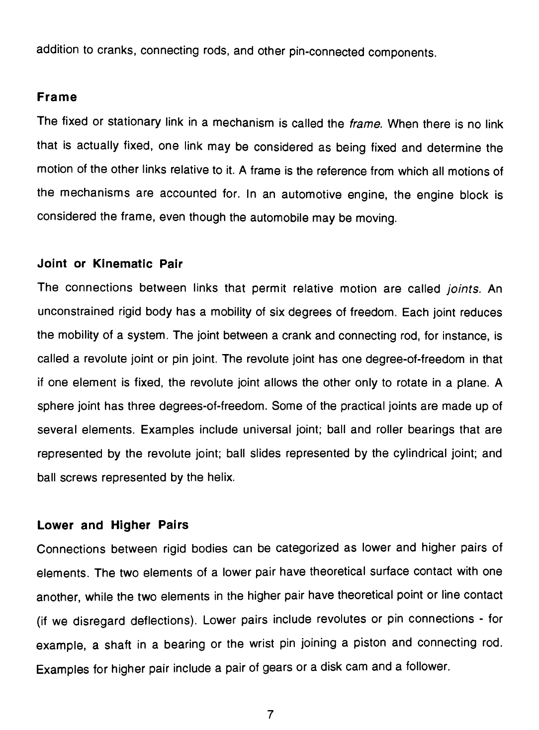
Frame
The
fixed
or
stationary
link
in
a
mechanism
is
called
the
frame.
When
there
is
no
link
that
is
actually
fixed,
one
link
may
be
considered
as
being
fixed
and
determine
the
motion
of
the
other
links
relative
to
it.
A
frame
is
the
reference
from
which
all
motions
of
the
mechanisms
are
accounted
for.
In
an
automotive
engine,
the
engine
block
is
considered
the
frame,
even
though
the
automobile
may
be
moving.
Joint
or
Kinematic
Pair
The
connections
between
links
that
permit
relative
motion
are
called
joints.
An
unconstrained
rigid
body
has
a
mobility
of
six
degrees
of
freedom.
Each
joint
reduces
the
mobility
of
a
system.
The
joint
between
a
crank
and
connecting
rod,
for
instance,
is
called
a
revolute
joint
or
pin
joint.
The
revolute
joint
has
one
degree-of-freedom
in
that
if
one
element
is
fixed,
the
revolute
joint
allows
the
other
only
to
rotate
in
a
plane.
A
sphere
joint
has
three
degrees-of-freedom.
Some
of
the
practical
joints
are
made
up
of
several
elements.
Examples
include
universal
joint;
ball
and
roller
bearings
that
are
represented
by
the
revolute
joint;
ball
slides
represented
by
the
cylindrical
joint;
and
ball
screws
represented
by
the
helix.
Lower
and
Higher
Pairs
Connections
between
rigid
bodies
can
be
categorized
as
lower
and
higher
pairs
of
elements.
The
two
elements
of
a
lower
pair
have
theoretical
surface
contact
with
one
another,
while
the
two
elements
in
the
higher
pair
have
theoretical
point
or
line
contact
(if
we
disregard
deflections).
Lower
pairs
include
revolutes
or
pin
connections
-
for
example,
a
shaft
in
a
bearing
or
the
wrist
pin
joining
a
piston
and
connecting
rod.
Examples
for
higher
pair
include
a
pair
of
gears
or
a
disk
cam
and
a
follower.

Kinematic Chain
A
kinematic
chain
is
an
assembly
of
links
and
joints.
In
a
closed
kinematic
chain,
e
link
is
connected
to
two
or
more
other
links.
Mechanism
A
mechanism
is
a
kinematic
chain
in
which
one
link
is
considered
fixed
for
the
purr.
of
analysis,
but
motion
is
possible
in
other
links.
As
noted
above,
the
link
design
as
the
fixed
link
need
not
actually
be
stationary
relative
to
the
surface
of
the
eart
kinematic
chain
is
usually
identified
as
a
mechanism
if
its
primary
purpose
is
modification
or
transmission
of
motion.
Linkage
If
kinematic
chains
are
needed
to
be
examined
without
regard
to
its
ultimate
use
assemblage
of
rigid
bodies
connected
by
kinematic
joints
of
lower
pairs
are
iden
as
a
linkage.
Thus,
both
mechanisms
and
machines
may
be
considered
link.
However
in
general,
the
term
linkage
is
restricted
to
kinematic
chains
made
lower
pairs.
Planar
Motion
and
Planar
Linkages
If
all
points
in
a
system
moves
in
parallel
planes,
then
that
system
undergoes
/
motion.
All
the
links
in
a
planar
linkage
have
planar
motion.
This
work
w
concerned
only
with
planar
linkages.
A
skeleton
diagram
of
a
planar
linkage
(e.c
Fig.
2.1)
is
formed
by
connecting
the
pin
centers
by
straight
lines
and
projecting
these
centerlines
on
one
of
the
planes
of
motion.
The
linkages
in
which
motion
(
be
described
as
taking
place
in
parallel
planes
are
called
spatial
or
three-dimer
(3D)
linkages.
8

Link
2
1
'////.
Link
3
3
'////.
Fig
2.1
A
Skeleton
Diagram
of
a
Planar
Linkage
Cycle
and
Period
A
cycle
represents
the
complete
sequence
of
positions
of
the
links
in
a
mechanism
(all
points
attained
between
two
identical
positions).
In
a
four-stroke-cycle
engine,
one
thermodynamic
cycle
corresponds
to
two
revolutions
or
cycles
of
the
crankshaft
but
one
revolution
of
the
camshaft
and,
thus,
one
cycle
of
motion
of
the
cam
followers
and
valves.
The
time
required
to
complete
a
cycle
of
motion
is
called
the
period.

3.
FOUR-BAR
MECHANISM
AND
ITS
CLASSIFICATIONS
An
important
property
of
a
classification
system
would
be
the
aid
it
could
furnish
a
designer
in
finding
the
forms
and
arrangements
best
suited
to
satisfying
certain
conditions.
The
planar
four-bar
mechanism
which
consists
of
four
pin-connected
rigid
links
gains
its
importance
as
a
basic
mechanism
because
it
is
one
of
the
simplest
of
all
mechanisms
to
produce.
The
four-bar
linkage
derives
its
renown
from
the
fact
that
the
members
of
a
three
bar
linkage
are
incapable
of
relative
motion
and
a
linkage
composed
of
more
than
four
bars
has
indeterminate
motion
with
a
single
input.
Though
it
may
assume
many
forms,
often
with
little
resemblance
to
the
usual
representation,
a
four-bar
linkage
consists
of
two
members
in
pure
rotation
about
fixed
axes,
called
the
driving
and
follower
crank;
a
coupler
in
combined
motion,
which
joins
the
moving
ends
of
the
cranks;
and
a
fixed
frame,
which
establishes
the
relative
position
of
the
stationary
crank
centers.
3.
1.
Classifications
and
the
Grashof
Criteria
There
are
two
main
classes
of
four
bar
mechanisms
based
on
the
rotational
and
dimensional
limitations
of
its
links
called
Grashof's
criterion,
which
are:
1.
Grashof
mechanisms,
which
is
comprised
of:
crank
rocker
mechanism
drag
link
mechanism
double
rocker
mechanism
crossover-position
or
change
point
mechanism
2.
Non-Grashof
Mechanisms,
which
includes
double
rocker
mechanisms
of
the
second
kind
or
triple
rocker
mechanisms.
10

A
Grashof
mechanism
is
a
four
bar
linkage
in
which
one
link
can
perform
a
complete
rotation
relative
to
the
other
three.
This
criterion
would
be
considered
if
we
plan
to
drive
a
linkage
with
a
continuously
rotating
motor.
It
will
be
shown
that
the
Grashof
criterion
is
met
if:
-max
+
Lmin
^
La
+
Lb
(3.1)
where
link
lengths
are
measured
between
bearing
centers,
Lmax
is
the
length
of
the
longest
link,
Lmjn
that
of
the
shortest
link,
La
and
Lb
are
the
lengths
of
the
remaining
links.
Fig.
3.1
Crank
Rocker
Mechanism
11

A
Grashof
mechanism
in
which
the
drive
crank
is
the
shortest
(and
Lmax
+
Lmjn
<
La
+
Lb)
will
act
as
a
crank
rocker
mechanism.
In
Figure
3.1,
the
skeleton
diagram
represents
a
crank
rocker
mechanism
where
link
0
represents
the
frame,
links
1
and
3
are
the
side
links
and
link
2
is
the
coupler.
The
smallest
side
link,
link
1,
often
acts
as
a
driving
crank.
The
rocker
link
(link
3)
will
oscillate
while
the
crank
(link
1)
is
rotated
continuously
in
one
direction.
Fig.
3.2
Drag
Link
Mechanism
12

A
Grashof
mechanism
in
which
the
fixed
link
is
the
shortest
(
and
Lmax
+
Lmjn
<
La
+
Lb)
will
act
as
a
drag
link
mechanism,
(see
Figure
3.2).
The
drive
crank
will
rotate
through
360
along
with
the
coupler
and
follower
crank.
A
Grashof
mechanism
in
which
coupler,
the
link
opposite
to
the
fixed
link,
is
shortest
and
Lmax
+
Lmjn
<
La
+
Lb
will
act
as
a
double
rocker
mechanism,
(see
Figure
3.3).
This
is
sometimes
called
double
rocker
of
the
first
kind.
Although
the
coupler
can
rotate
360,
neither crank
can
rotate
through
360.
In
a
linkage
of
this
type,
the
coupler
can
be
used
as
the
drive
member.
Figure
3.3
A
Double
Rocker
Mechanism
13

A
Grashof
mechanism
in
which
Lmax+
Lmjn
=
La
+
Lb
may
be
considered
a
crossover-position
or
change
point
mechanism.
Relative
motion
of
a
crossover
position
may
depend
on
inertia,
spring
forces,
or
other
forces
when
links
become
collinear.
Any
of
the
above
classes
of
linkages
may
be
driven
by
rotation
of
the
coupler
(the
link
opposite
the
fixed
link),
although
the
range
of
coupler
in
some
cases
may
be
very
limited.
The
coupler
effectively
provides
a
hinge
with
a
moving
center.
The
coupler-
driven
linkages
may
be
called
polycentric.
Four-bar
mechanisms
that
do
not
satisfy
the
Grashof
criterion,
Lmax
+
Lmjn
<
La
+
Lb
are
called
double
rocker
mechanisms
of
the
second
kind
or
triple
rocker
mechanisms.
In
this
case
no
link
can
rotate
through
360.
3.
2.
Proof
of
Grashof
Criteria
To
show
the
validity
of
the
Grashof
criteria,
we
may
begin
by
examining
a
crank
rocker
mechanism.
Referring
to
Figure
3.1
,
we
observe
that
the
range
of
motion
of
link
3
is
limited.
The
limiting
positions
of
link
3
occur
when
links
1
and
link
2
are
collinear.
The
linkage
arranges
itself
in
the
form
of
a
triangle.
Using
the
triangle
inequality,
we
obtain
the
required
relationships
between
lengths
of
the
crank
rocker
mechanism.
First,
using
Figure
3.4,
we
have
an
inequality
relating
the
length
of
the
fixed
link
to
the
others:
L0
<
L2
-
Li
+
L3
(3.2)
14

Figure
3.4
A
Limiting
Position
of
Crank
Rocker
Mechanism
Next,
a
similar
expression
is
obtained
for
follower
crank
3:
L3
<
L2
-
Li
+
Lq
(3.3)
Figure
3.5
Another
Limiting
Position
of
Crank
Rocker
Mechanism
15

From
Figure
3.5,
The
length
of
link
1
added
to
link
2
is
related
to
the
others
to
form
inequality:
Lt
+
L2
<
Lq+
L3
(3.4)
Combining
inequalities
3.2,
3.3
and
3.4,
we
have
L1+
IL2-L3I
<
L0
<
L<\
+
L3
(3.5)
Actually,
there
are
three
additional
possible
inequalities
based
on
the
triangle
formed
in
Figure
3.5,
but
these
three
inequalities
are
redundant.
Inequalities
3.2
and
3.3,
respectively,
may
be
written
in
the
following
form:
L-|
<
-
L0
+
L2
+
L3
(3.6)
1-1
<
L0
+
L2
"
L3
(3.7)
In
this
from,
the
inequalities
may
be
added
to
obtain
2
L-|
<
2
L2
or
L-j
<
L2
(3.8)
Similarly
using
inequality
3.2
and
3.4,
we
have
Li
<
L3
(3.9)
Using
3.3
with
3.4,
we
have
16

L1
<
L0
(3.10)
Thus,
if
the
driver
crank
(which
we
label
link
1)
is
the
shortest
link
in
a
four-bar
mechanism,
we
may
have
a
crank
rocker
mechanism.
If
inequalities
3.2,
3.3
and
3.4
are
satisfied
for
the
given
mechanism,
the
identification
of
the
mechanism
as
a
crank
rocker
mechanism
is
then
positive;
link
3
will
oscillate
as
link
1
rotates
continuously.
Substituting
Lmjn
for
L-|
and
Lmax
for
each
of
Lq, L2,
and
L3
in
turn,
in
inequality
3.5,
we
see
that
it
is
identical
to
the
more
concise
requirements
for
a
crank
rocker
mechanism:
(a)
Lmax
+
Lmjn
<
La
+
Lb
and
(b)
the
crank
is
the
shortest
link.
If
link
0,
the
fixed
link,
is
shortest,
as
in
the
drag
link
mechanism,
we
may
substitute
Lq
for
L-j,
L-|
for
L2
,
L2
for
L3
and
L3
for
Lq
in
inequality
3.2
to
obtain
L0
+
ll_-|
-L2I
<
L3
<
L-|
-
L0
+
L2
(3.11)
If
link
2,
the
coupler
link,
is
shortest,
as
in
a
double
rocker
mechanism,
by
similar
permutation,
we
obtain
L2
+
IL3-L0I
<
L-l
<
L3
-
L2
+
L0
(3.12)
Substituting
as
we
did
in
inequality
3.5
we
see
that
in
equalities
3.1
1
and
3.12
satisfy
the
Grashof
inequality:
Lmax
+
Lmin
<
La
+
Lb
(3-13)
Each
of
these
mechanisms
may
be
considered
as
inversion
of
the
others.
Four-bar
17

linkages
that
violate
the
Grashof
criteria
are
triple
rocker
mechanisms.
Each
Grashof
mechanism
has
two
assembly
configurations.
The
positions
attainable
in
one
assembly
configuration
are
not
attainable
in
the
other.
A
summary
of
the
results
is
given
in
Table
3.1.
Table
3.
1.
Summary
of
the
Criteria
of
Motion
for
Each
Class
of
Four-Bar
Linkages
l-min:
Lmax:
La
and
Lb:
shortest
link;
longest
link;
links
of
intermediate
links
Type
of
Mechanism
Shortest
Link
Relationship
Between
Links
GRASHOF
Any
-max
+
Lmin
-
La
+
Lb
Crank
rocker
Driver
crank
Lmax
+
Lmin
<
La
+
Md
Drag
link
Fixed
link
Lmax
+
Lmin
<
La
+
Lb
Double-rocker
Coupler
Lmax
+
Lmin
<
La
+
Lb
Crossover-position
Any
Lmax
+
Lmin
=
La
+
Lb
NON-GRASHOF
Triple-rocker
Any
Lmax
+
Lmin
>
La
+
Lb
18

4.
SPECIAL
FOUR-BAR
MECHANISMS
FOR
APPROXIMATE
STRAIGHT
LINE
OUTPUT
One
of
the
special
applications
of
four-bar
linkages
is
as
function
generators.
The
atlas,
Analysis
of
the
four-bar
linkage,
by
Hrones
and
Nelson,
contains
a
few
coupler
curves
with
approximate
straight
lines
that
have
been
useful
for
practical
design
problems.
Four
well-known
four-bar
linkages
which
are
capable
of
generating
straight
line
motion
will
be
introduced
in
this
chapter.
However,
those
mechanisms
given
by
the
atlas
are
inflexible
in
design,
and
only
occasionally
they
fit
the
problems
the
designers
face
in
practice;
in
most
cases
to
suit
particular
needs
mechanisms
for
straight
line
motions
needed
to
be
developed.
In
this
chapter,
these
four
mechanisms
will
be
categorically
defined
and
their
mobility
will
be
investigated.
4.
1.
Evans
Linkage
Evans
Linkage
is
a
crank
rocker
mechanism
in
which
the
crank
L-|
rotates
through
a
Fig
4.1
Evans
Linkage
19
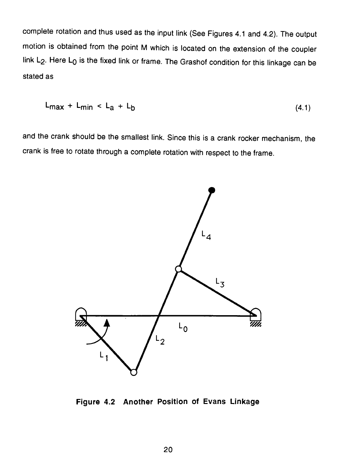
complete
rotation
and
thus
used
as
the
input
link
(See
Figures
4.1
and
4.2).
The
output
motion
is
obtained
from
the
point
M
which
is
located
on
the
extension
of
the
coupler
link
L2.
Here
L0
is
the
fixed
link
or
frame.
The
Grashof
condition
for
this
linkage
can
be
stated
as
Lmax
+
Lmjn
<
La
+
Lb
(4.1)
and
the
crank
should
be
the
smallest
link.
Since
this
is
a crank
rocker
mechanism,
the
crank
is
free
to
rotate
through
a
complete
rotation
with
respect
to
the
frame.
Figure
4.2
Another
Position
of
Evans
Linkage
20

4.
2.
Chebyshev
Linkage
Chebyshev
Linkage
is
a
four-bar
double
rocker
mechanism
where
the
coupler
rotates
through
360.
Figure
4.3
shows
a
schematic
diagram
of
the
Chebyshev
linkage.
In
Chebyshev's
Linkage
either
the
crank
or
the
coupler
can
be
used
as
the
input
link.
The
output
is
obtained
from
the
point
M
located
at
the
middle
of
the
coupler.
The
limiting
positions
of
the
crank
in
relation
to
the
frame
for
this
mechanism
are
shown
in
Figures
4.4
and
4.5.
Figure
4.3
Chebyshev
Linkage
The
conditions
for
Chebyshev's
Linkage
is
same
as
the
Grashof's
criteria:
Lmax
+
Lmin
<
La
+
Lb
(4.2)
and
the
smallest
link
is
the
coupler
L2.
The
limiting
angles
between
the
crank
and
the
frame
for
Chebyshev's
Linkage
are
calculated
using
cosine
law
(refer
Figure
4.4).
21

o
'////*
Figure
4.4
Limiting
Angle
of
Chebyshev
Linkage
By
cosine
law:
(L3
-
L2)2
=
|_02
+
Li
2
-
2
L0
L^
cos
0min
=>
Qmin
=
cos-1
{
[
L02
+
L^
-(L3-
L2)2
]/2
L0
L-\
}
(4.3)
Figure
4.5.
Another
Limiting
Angle
of
Chebyshev
Linkage
Similarly
to
calculate
0max
from
Figure
4.5,
22

=>
(L3
+
L2)2
=
L02
+
L-|2-2
Lq
L-|
cos
6max
6max
=
cos-1{[L02
+
L12-(L3
+
L2)2]/2L0L1}
(4.4)
4.
3.
Watts
Linkage
A
pictorial
representation
of
Watts
Linkage
(refer
Figure
4.6)
resembles
that
of
the
Chebyshev's.
But
it
differs
from
Chebyshev's
by
the
fact
that
it
is
not
a
double
rocker
mechanism
which
means
no
link
in
this
mechanism
rotates
through
360.
The
limiting
positions
of
the
crank
for
this
mechanism
are
shown
in
Figures
4.7
and
4.8.
Figure
4.6
Watts
Linkage
Being
a
non-Grashof
mechanism,
Watts
Linkage
does
not
satisfy
the
Grashof
Criteria.
The
condition
for
this
kind
of
link
mechanism
is,
Lmax
+
Lmin
>
La
+
Lb
(4.5)
23

Figure
4.7
Limiting
Position
of
Watts
Linkage
Figure
4.7
will
show
that
the
limiting
angle
emax
for
Watts
Linkage
can
be
calculated
as
same
way
as
that
of
Chebyshev's.
(I_3
+
L2)2
=
L02
+
Li
2
-
2
Lq
L<[
COS
6max
=>
emax
=
COS-1{[L02
+
L12-(L3
+
L2)2]/2LoL1}
(4.6)
and
in
this
case,
fynin
-
~
^max
(4.7)
Figure
4.8
The
Other
Limiting
Position
of
Watts
Linkage
24

4. 4.
Roberts
Linkage
Roberts
Linkage
is
a
mechanism
of
triple
rocker
kind
in
which
none
of
the
links
rotate
through
360.
Figure
4.9
shows
a
Roberts
mechanism.
Figure
4.9
Roberts
Linkage
From
the
limiting
positions
illustrated
by
Figure
4.10,
by
cosine
law,
L32
=
L02
+
(Lt
+
L2)2
-
2
L0
(Li
+
L2)
cos
emin
=>
emin
=
cos-1
{
[
L02
+
(Li
+
L2)2
-
L32
]
/
2
L0
(Li
+
L2)
}
(4.8)
25

Figure
4.11
The
Limiting
Positions
of
Roberts
Linkage
26

and
0max
is
calculated
as,
(L2
+
L3)2
=
Lq2
+
Li2
-
2
Lq
Li
cos
6max
=>
max
=
cos-1
{
[
Lq2
+
L^
-
(L2
+
L3)2
]
/
2
L0
Li
}
(4.9)
27

5.
POSITION
ANALYSIS
OF
A
BASIC
FOUR-BAR
MECHANISM
When
mechanisms
are
analyzed
both
graphical
and
analytical
methods
can
be
useful.
When
position
of
a
point
or
set
of
points
are
to
be
determined
for
a
single
linkage
position,
graphical
methods
are
usually
more
convenient.
Analytical
methods
are
more
practical
when
a
sequence
of
positions
of
a
mechanism
must
be
analyzed.
The
use
of
a
computer
permits
a
detailed
study
of
a
full
cycle
of
motion.
Once
the
initial
programming
is
completed,
little
effort
is
required
to
examine
the
effect
of
design
changes.
On
the
other
hand,
if
we
were
to
use
graphical
methods,
each
linkage
position
would
require
a
separate
plot
and
each
change
in
length
of
a
link
would
require
a
new
sequence
of
plots.
This
chapter
deals
with
the
analytical
method
of
determining
the
positions
of
the
links
relative
to
one
another.
Methods
of
vector
analysis
are
important
tools,
which
could
be
used
for
mechanism
analysis
and
synthesis.
5.1
Vectors
Vectors
provide
graphical
and
analytical
means
to
represent
motion.
A
quantity
described
by
its
magnitude
and
direction
can
be
considered
a
vector
and
can
be
graphically
represented
by
an
arrow.
The
length
of
the
arrow
is
proportional
to
the
magnitude
of
the
vector
quantity
and
the
direction
of
the
arrow
is
the
direction
of
the
vector
quantity.
Graphical
and
analytical
vector
methods
can
be
applied
to
linear
displacements,
velocities,
accelerations
and
forces,
and
to
torques
and
angular
velocities
and
accelerations.
Vectors
will
be
identified
in
this
study
by
boldface
type
to
distinguish
from
scalar
quantities.
28

In
general,
a
vector
of
unit
magnitude
can
be
called
a
unit
vector.
Thus,
A^
=
A
/
A
is
a
unit
vector
in
the
direction
of
A,
where
A
=
IAI
is
the
magnitude
of
vector
A.
A
coordinate
system
in
which
the
axes
are
mutually
perpendicular
is
called
a
rectangular
coordinate
system.
Unit
vectors
i,
j,
k
parallel
to
the
x, y,
z
coordinate
axes,
respectively,
are
particularly
useful,
since
we
are
going
to
use
only
rectangular
coordinate
system
throughout
this
work.
These
unit
vectors
are
also
called
rectangular
unit
vectors.
A
vector
may
be
described
in
terms
of
its
components
along
each
coordinate
axis.
When
we
use
vectors
to
describe
the
motion
of
a
linkage,
it
is
advisable
to
make
a
sketch
of
the
linkage
adjacent
to
vector
diagrams
so
that
vector
directions
can
be
referred
to
linkage
orientation.
5.
1.
1
Solution
Of
Planar
Vector
Equations
Consider
the
planar
vector
equation
A
+
B
+
C
=
0
or
in
terms
of
unit
vectors
(Au
etc.)
and
magnitudes
(A
etc.),
AU
A
+
BU
B
+
CU
C
=
0
If
the
magnitude
and
direction
of
the
same
vector
are
unknown,
then
the
solution
is
easily
obtained.
If
C
is
unknown,
we
use
C
=
-
(
Ax
+
Bx
)
i
-
(
Ay
+
By
)
j
or
C
=
-(Ai
+
B
i
)
i
-
(Aj
+
B
*
j
)
j
If
the
magnitudes
of
two
different
vectors
are
unknown,
a
vector
elimination
method
may
be
used.
Suppose,
for
example,
magnitudes
A
=
I
A
I
and
B
=
I
B
I
are
unknown
in
29

the
vector
equation
AU
A
+
BU
B
+
Cu
C
=
0.
We
take
the
dot
product
of
each
term
with
BU
x
k
noting
that
Bu
(
bu
x
k
)
=
0
since
vector
BU
is
perpendicular
to
vector
BU
X
k.
Thus,
we
obtain
AUA(BUXk)
+
C-(BUXk)
=
0
from
which
the
magnitude
of
vector
A
is
given
by
-C(BUXk)
A=
(5.1)
AU.(BUXk)
Similarly,
the
magnitude
of
B
is
given
by
-
C
(
AU
x
k
)
B
=
(
5.2
)
BU
(
AU
X k
)
If
the
vector
directions
Au
and
Bu
are
unknown
but
all
vector
magnitudes
are
known,
the
solution
to
the
equation
A
+
B
+
C
=
0
is
more
difficult.
The
results
in
this
case,
as
given
in
Reference
1
0,
are
A
=
_{B2
-[(c2
+
B2-A2)/2C]2}(1/2)
(CUXk)
+
{
[
(C2
+
B2
-
A2)/2C
]
-
C
}
CU
(5.3a)
or
A
=
+
{B2
-[(C2
+
B2-A2)/2C]2}(1/2)
(CU
X
k
)
+
{
[
(C2
+
B2
-
A2)/2C
]
-
C
}
CU
(5.3b)
and
B
=
+
{B2
-
[
(
C2
+
B2
-
A2
)/2C
]2
}(1/2)
(Cu
x
k
)
+
[
(C2
+
B2
-
A2)/2C
]
CU
(5.4a)
or
B
=
-{B2
-[(C2
+
b2-A2)/2C]2}(1/2)
(C"
X
k
)
+
[
(C2
+
B2
-
A2)/2C
]
CU
(5.4b)
30

When
the
magnitude
of
A
and
the
direction
of
B
are
unknown,
A
and
B
may
be
found
by
the
following
equations:
A
=
{
-
C
AU
V
B2
-
[
C
(
AU
X
k
)]2
}
AU
B
=
-
[
C
(
AU
X
k)
]
(
AU
x
k)
V
B2
-
[
C
(
AU
X
k
)]2
}
AU
(5.5)
(5-6)
The
above
approach
uses
vector
notation
throughout,
unlike
alternate
methods
that
use
vector
analysis
to
derive
scalar
equations.
When
the
above
method
is
used
for
computer-aided
analysis
and
design
of
mechanisms,
computer
subroutines
will
be
incorporated
to
handle
the
conversion
from
vector
to
scalars.
The
above
equation
will
be
applied
to
the
analysis
of
planar
linkages.
Figure
5.1
A
Basic
Four-Bar
Planar
Linkage
31

5.
2
The
Four
Bar
Linkage
A
graphical
layout
of
a
four
bar
linkage
can
be
easily
constructed.
We
only
require
to
know
the
position
of
one
link
be
given
in
relative
to
the
frame
and
the
link
lengths.
One
such
layout
for
the
simplest
four
bar
mechanism
is
given
in
Fig.
5.1.
Analytical
formulas
are
to
be developed
to
determine
all
the
link
positions
needed
to
write
a
computer
program.
The
following
analysis
provides
an
analytical
solution
for
a
simple
mechanism
shown
as
vector
notations
in
Fig.
5.2
and
this
can
be
modified
to
suit
the
different
kinds
of
four
bar
mechanisms
in
the
later
parts
of
this
chapter.
Note
that
there
are
two
different
modes
of
assembly
possible
for
a
non-Grashof
mechanism.
(Refer
Chapter
3).
Figure
5.2
Vector
Representation
of
a
Planar
Four-Bar
Linkage
32

5. 2.
1
Position
Analysis
Using
Vector
Cross
Product
Equations
5.3
and
5.4
may
be
used
to
find
linkage
displacements.
These
equations
apply
when
directions
of
vectors
A
and
B
are
unknown.
The
four
bar
planar
linkage
of
Fig.
5.2
is
described
by
the
vector
equation
r0
+
n
+
r2
+
r3
=
0
or
rd
=
-
(
r2
+
r3
)
where
the
diagonal
is
given
by
rd
=
r0
+
ri
If
the
lengths
of
the
links
are
specified
and
orientation
of
link
1
is
given,
then
the
following
substitution
may
be
made
in
equations
5.3
and
5.4:
A
=
r2
B
=
r3
C
=
rd=
r0
+
ri
yielding,
if
the
linkage
is
assembled
so
that
the
vector
loop
r2r3rd
is
clockwise
as
in
Fig.
5.2,
r2
=
-{r32
-
[(r32-r22
+
rd2)/(2rd)]2}1/2
(rduXk)
+
[(r32-r22
+
rd2)/(2rd)
-
rd
]
rdu
(5.7)
r3
=
+{r32
_
[(r32_r22
+
rd2)/(2rd)]2}1/2
(rduXk)
-
[(r32-r22
+
rd2)/(2rd)
-
rd
]
rdu
(5.8)
and
if
the
vector
loop
r2r3rd
is
counterclockwise
as
in
Fig.
5.3,
33

Figure
5.3
Vector
Representation
of
a
Four-Bar
Linkage
(Alternative
Mode
of
Assembly)
r2
=
+{r32
-
[(r32-r22
+
rd2)/(2rd)]2}1/2
(rduXk)
+
[(r32-r22
+
rd2)/(2rd)
-
rd
]
rdu
(5.9)
r3
=
-{r32
-
[(r32-r22
+
rd2)/(2rd)]2}1/2
(rduXk)
-
[(r32-r22
+
rd2)/(2rd)
-
rd
]
rdu
(5.10)
In
order
to be
used
in
a
computer
program,
analytical
formulas
are
to
be
developed
for
different
link
positions.
These
formulas
can
be
developed
using
the
concepts
of
vector
operations
and
incorporating
them.
34

6.
EQUATION
OF
COUPLER
CURVE
OF
A
GENERIC
FOUR
BAR
LINKAGE
In
order
to
investigate
algebraically
the
function
generated
by
a
coupler
point,
a
generic
equation
of
this
coupler
curve
should
be
obtained.
The
equation
of
the
coupler
point
curve
for
a
four-bar
linkage
was
first
derived
by
Samuel
Roberts
by
using
analytic
geometry.
The
equation
will
be
written
in
Cartesian
coordinates,
with
x
axis
along
the
line
of
centers
OaOb
and
the
y
axis
perpendicular
to
that
line
at
Oa
(See
Fig.
6.1).
Let
(x-|,yi),
(x2,y2),
and
(x,y)
be,
respectively,
the
coordinates
of
points
A,
B
and
coupler
point
M;
then
x-|
=
x
-
b
cos
9
yi
=
y
-
b
sin
e
and
x2
=
x-acos(e
+
y)
y2
=
y-asin
(6
+
y)
(6.1)
Since
A
and
B
describe
circles
(or
arcs
of
circles)
about
centers
Oa
and
Ob,
respectively,
Xl2
+
yi2
=
r2
and
(x2
-
p)2
+
y22
=
s2
(6.2)
Substituting
the
values
of
x-|,yi
and
x2,y2
into
the
last
two
equations
yields,
(x
-
b
cos
e)2
+
(y
-
b
sin
6)2
=
r2
and
[x-acos(e
+
y)-p]2
+
asin(e
+
y)]2
=
s2
(6.3)
which,
by
application
of
trigonometric
identities,
ordering
of
terms
and
simplification,
become:
35

B
Figure
6.1
A
Graphical
Layout
of
a
Generic
Four-Bar
Linkage
36

x
cos
0
+
y
sin
0
=
(x2
+
y2
+
b2
-
r2)
/
2
b
and
[
(x
-
p)
cos
y
+
y
sin
y
]
cos
0
-
[
(x
-
p)
sin
y
-
y
cos
y
]
sin
0
=
[(x-p)2
+
y2
+
a2-s2]/2a
(6.4)
The
equation
of
the
coupler-point
curve
may
now
be
obtained
by
elimination
of
0
between
the
last
two
equations.
Solving
these
equations
for
cos
0
and
sin
0
and
substituting
the
values
obtained
into
identity
cos2
0
+
sin2
0
=
1
yields
the
general
four-bar
coupler
curve
equation:
{
sin
a
[(x
-
p)
sin
y
-
y
cos
y
]
(x2
+
y2
+
b2
-
r2)
+
y
sin
p
[(x
-
p)2
+
y2
+
a2
-
s2]}2
+
{
sin
a
[(x
-
p)
cos
y
+
y
sin
y
]
(x2
+
y2
+
b2
-
r2)
-
x
sin
(3
[(x
-
p)2
+
y2
+
a2
-
s2]}2
=
4
k2
sin2
a
sin2
p
sin2
y
[x
(x
-
p)
-
y2
-
p
y
cot
y
]2
(6.5)
In
this,
k
is
the
constant
of
the
sine
law
applied
to
the
triangle
ABM,
a
b
c
sin
a
sin
p
sin
y
This
equation
is
of
the
sixth
degree
because
one
of
its
property
is
that
a
straight
line
will
intersect
it
in
no
more
than
six
points.
In
the
following
sections
the
equation
of
motion
of
specific
four-bar
mechanisms
will
be
derived
in
a
similar
approach.
37

7.
FOUR-BAR
MECHANISMS
THAT
GENERATE
SYMMETRICAL
COUPLER
CURVES
Symmetrical
curves
generated
by
a
four-bar
mechanism
have
received
a great
deal
of
attention
due
to
their
wide
applications.
In
this
chapter
conditions
for
a
four-bar
mechanism
to
produce
a
symmetrical
coupler
curve
will
be
discussed.
The
following
theorem
and
proof
were
presented
by
Berzak
(Reference
8
and
9).
Symmetrical
Coupler
Curves
Let
a
symmetrical
four-bar
mechanism
be
defined
as
a
four-bar
mechanism
for
which
the
length
of
the
crank
and
the
length
of
the
rocker
are
equal.
Theorem
1:
In
a
symmetrical
four-bar
mechanism,
any
point
in
the
coupler
plane
which
lies
on
the
perpendicular
bisector
of
the
coupler,
generates
a
symmetrical
curve,
with
the
perpendicular
bisector
of
the
frame
as
a
line
of
symmetry.
Proof
of
Theorem
1
Using
Analytical
Geometry
The
equation
of
the
coupler
curve
generated
by
point
M
of
the
four
bar
mechanism
shown
in
Fig.
7.1
is
given
by
the
equation
7.1.
This
equation
was
first
derived
by
Samuel
Roberts
and
is
presented
with
slight
modifications.
The
derivation
of
this
equation
is
explained
in
Chapter
6.
The
equation
is
written
in
Cartesian
coordinates
with
origin
at
the
center
of
rotation
of
the
crank
Oa,
and
x-axis
along
OaOb,
where
Ob
is
the
center
of
rotation
of
rocker.
38

B
Figure
7.1
Graphical
Layout
of
a
Four-Bar
Mechanism
39

{
sin
a
[(x
-
p)
sin
y-
y
cos
y]
(x2
+
y2
+
b2
-
r2)
+
ysinp
[(x-p)2
+
y2
+
a2-s2]}2
+
{
sin
a
[(x
-
p)
cos
y+
y
sin
y
]
(x2
+
y2
+
b2
-
r2)
-xsinp
[(x-p)2
+
y2
+
a2-s2]}2
=
4k2sin2a
sin2
p
sin2Y
[x
(x-p)
-y2
-p
y
cot
y]2
(7.1)
In
this,
k
is
the
constant
of
the
sine
law
applied
to
the
triangle
ABM,
a
b
c
k
=
=
=
sin
a
sin
p
sin
y
All
angles
in
this
are
positive
when
measured
in
the
counter
clockwise
direction.
A
special
four-bar
mechanism
is
shown
in
Fig.
7.2.
For
this
mechanism:
r
=
s
(7.2)
In
view
of
the
choice
of
point
M,
triangle
ABM
is
isosceles.
Therefore:
a
=
b
and
a
=
p
(7.3)
From
the
condition
that
the
sum
of
the
angles
in
a
triangle
is
180
together
with
equation
7.3
the
following
conditions
are
obtained.
sin
a
=
sin
2p
(7.4a)
cos
a
=
cos
2p
(7.4b)
Substituting
these
into
equation
7.1,
we
get
40

Figure
7.2
A
Symmetric
Linkage
41

{
sin
p
[
(
x
-
p
)
sin
2
p
+
y
cos
2
p
]
(
x2
+
y2
+
b2
-
r2
)
+
y
sin
p
[
(
x
-
p
)2
+
y2
+
b2
-
r2
]
}2
+
{
sin
p
[
(
x
-
p
)
(
-
cos
2
p
)
+
y
sin
2
p
]
(
x2
+
y2
+
b2
-
r2
)
-
x
sin
b
[
(
x
-
p
)2
+
y2
+
b2
-
r2
]
J2
=
4k2sin4psin22p[x(x-p)-y2
+
pycot2p]2
(7.5)
Now
if
we
will
transform
the
equation
to
a
new
X,Y
coordinate
system.
The
origin
of
this
coordinate
system
is
at
the
center
of
the
frame.
The
X-axis
coincides
with
the
x-axis,
and
X,Y
coordinate
system
is
also
right-handed.
The
transformation
equations
are
defined
by
the
equations:
x
=
X
+
p/2
and
y
=
Y
(7.6)
Substitution
of
these
transformation
into
equation
7.5
results
in,
X6
sin22p
+
X4
[
p2
sin2p
(1-3
cos2p
)
+
2
sin22p
(
b2
-
r2
)
-4
b2
sin22P
sin2p
]
-
2
X*
Y
p
sin2p
sin
2p
+
3
X* Y2
sin22p
+
X2
[
(
p4
/
4
)
sin2p
(1-3
sin2p
)
-
2
p2
(
b2
-
r2
)
sin2p
+
(
b2
-
r2
)2
sin22p
+
2
b2
p2
sin2p
sin22p
]
+
X2
Y
{
p
sin
2p
[
sin2p
(
p2
-
4
b2
+
4
r2
)
-8
b2
cos
2P
sin2p
j
}
+
X2
y2
[
2
p2
sin4p
-
8
b2
sin2p
sin22p
+
4
(
b2
-
r2
)
sin22p
]
-
4
X2
y3
p
sin
2p
sin2p
+
3
X2
Y^
sin22p
+
Y6
sin22p
-
2
Y5
p
sin
2p
sin2p
+
Y^
[
2
sin22p
(
b2
-
r2
)
+
p2
sin2p
(
1
+
cos2p
)
-
4
b2
sin2p
sin22p]
+
Y3
[
p
sin
2P
sin2p
(
-
p2
-
4
b2
+
4
r2
)
-
8
b2
p
sin
2P
sin2p
cos
2p
]
42

+
Y2[(p4/4)sin2p(1+sin2p
+
(b2-r2)2sin22p
+
2p2(b2-r2)sin2p
-
4
b2
p2
sin2p
(1-6
cos2p
+
6
cos4p
)
]
+
Y{(p/2)sin2psin2P[-p4/4-4(b2-r2)2-2p2(b2-r2)]
+
2
b2
p3
sin
2p
cos
2p
sin2p
}
+
p2
sin4p
[
(
p4
/
1
6
)
+
(
b2
-
r2
)2
+
(
p2
/
2
)
(
b2
-
r2
)
]
-
(
1
/
4
)
b2
p4
sin22p
sin2p
=
0
(7.7)
A
close
examination
of
the
above equation
will
show
that
all
coefficients
of
odd
powers
of
X
are
zero,
which
follows
that
the
Y-axis
coincides
with
the
line
of
symmetry
of
the
coupler
curve.
The
following
theorem
and
proof
are
presented
by
Hartenberg
and
Denavit,
in
Reference
1.
Theorem
2:
Coupler
curves
that
are
symmetrical about
an
axis
may
be
generated
by
a
four
bar
linkage
with
a
coupler
base
AB
and
follower OgB
of
equal
length.
The
coupler
point
must
lie
anywhere
on
the
circle
centered
at
B
and
passing
through
A
(refer
figure
7.3).
Since
BOb
=
BA
=
BM,
the
above
circle
also
passes
through
Ob
and
the
inscribed
angle
AObM
satisfies
the
relation
<AObM
=
<ABM/2
=
p/2
=
constant.
(7.8)
Consider
now
the
linkage
in
two
positions
OaA-|B-|Ob
and
OaA2B2Ob
for
which
points
Ai
and
A2
are
symmetrical
with
respect
to
the
line
of
fixed
centers
OaOb
(Figure
7.4).
For
these
positions,
triangles
ObA-|Bi
and
ObA2B2
are
equal,
since
43

corresponding
sides
are
equal,
whence
pi
=
P2.
0
B
Figure
7.3
A
Four-Bar
Mechanism
That
Generates
Symmetrical
Coupler
Curves
44

Figure
7.4
Two
Positions
of
a
Four-Bar
Corresponding
to
Symmetrical
Points
M-\
and
M2
on
the
Coupler
Curve
45

Now,
the
isosceles
triangles
ObB-|Mi
and
ObB2M2
are
equal,
ObMi
=
ObM2
(7.9)
and
the
midnormal
c
to
MiM2
passes
through
Ob
and
bisects
the
angle
M1ObM2,
whence
8
+
y
=
a
+
p/2
(710)
Since
the
angles
OaObAi
and
OaObA2
are
also
equal
(A-|
symmetric
to
A2
with
respect
to
OaOb),
Y+
a
=
p/2
+
8
(7.11)
Adding
the
last
two
equations
yields
Y
=
0/2
(712)
The
midnormal
c
to
M-|M2,
therefore
makes
a
constant
angle
with
the
line
of
fixed
centers
OaOb,
whence
it
is
an
axis
of
symmetry
for
the
coupler
curve
generated
by
point
M.
It
should
further
be
noted
that
symmetric
points
on
the
coupler
curve
corresponds
to
symmetric
positions
of
the
crank
with
respect
to
the
line
of
fixed
centers
OaOB-
46

8.
ANALYSIS
OF
FOUR-BAR
LINKAGES
GENERATING
STRAIGHT
LINE
COUPLER
CURVE
When
James
Watt
built
a
steam
engine
in
1769,
he
had
to
design
a
linkage
to
guide
a
pin
along
a
straight
line
path,
since
there
were
no
machine
tools
at
that
time
capable
of
producing
straight
metal
slides
of
sufficient
precision.
Since
then
straight
line
mechanisms
have
found
numerous
applications.
Straight
line
mechanisms
are
not
of
historic
interest
alone,
however,
since
four
bar
mechanisms
have
their
own
advantages
over
the
conventional
slides.
Many
four-bar
mechanisms
that
generate
approximate
straight
line
motion,
have
been
designed
in
the
past.
Although
they
have
proven
to
be
very
useful
for
practical
design
problems,
these
"ready-made"
straight
line
motions
only
occasionally
fit
the
design
problems
in
practice;
in
most
cases
the
designer
must
develop
straight
line
motion
to
suit
his/her
particular
needs.
This
chapter
derives
the
necessary
condition
to
obtain
a
straight
line
output
from
four
bar
mechanisms,
in
order
to
aid
the
designer
in
designing
his/her
mechanism
for
straight
line
motion
to
fit
his/her
needs.
8.
1
Evans
Linkage
A
schematic
layout
of
symmetrical
Evans
linkage
is
shown
in
Fig.
8.1.
From
Chapter
7,
we
are
now
aware
that
for
a
symmetric
coupler
curve
in
the
standard
Evans
linkage
(refer
Fig.
4.1)
the
values
of
s
,
a
and
b
must
be
equal
and
the
Fig.
8.1.
is
shown
as
such.
The
x-axis
is
drawn
along
the
frame
OaOb
and
the
y-axis
perpendicular
at
Oa-
Let
(x-i.yi),
(x2,y2)
and
(x,y)
be
respectively,
the
coordinates
of
points
A,
B
and
the
coupler
point
M;
then
47

B
x.X
Figure
8.1
Graphical
Layout
of
Symmetrical
Evans
Linkage
48
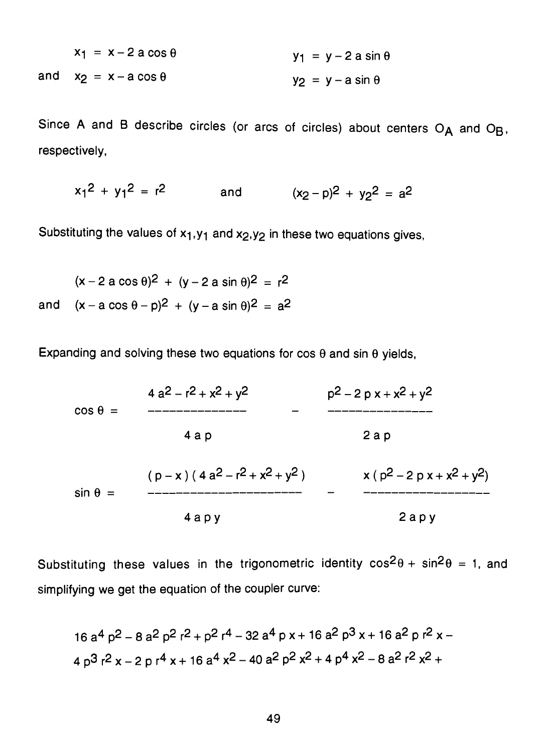
x-|
=
x
-
2
a
cos
6
yi
=
y
-
2
a
sin
6
and
x2
=
x
-
a
cos
9
y2
=
y
-
a
sin
e
Since
A
and
B
describe
circles
(or
arcs
of
circles)
about
centers
Oa
and
Ob,
respectively,
X12
+
yi2
=
r2
and
(X2
_
p)2
+
y22
=
a2
Substituting
the
values
of
x-|,yi
and
x2,y2
in
these
two
equations
gives,
(x-2acos0)2
+
(y-2asin9)2
=
r2
and
(x
-
a
cos
0
-
p)2
+
(y
-
a
sin
8)2
=
a2
Expanding
and
solving
these
two
equations
for
cos
9
and
sin
0
yields,
4
a2
-
r2
+
x2
+
y2
p2
-
2
p
x
+
x2
+
y2
cos
0
=
-
4
a
p
2
a
p
(
p
-
x
)
(
4
a2
-
r2
+
x2
+
y2
)
x
(
p2
-
2
p
x
+
x2
+
y2)
sin
0
=
-
4apy
2
apy
Substituting
these
values
in
the
trigonometric
identity
cos20
+
sin20
=
1,
and
simplifying
we
get
the
equation
of
the
coupler
curve:
16
a4
p2
-
8
a2
p2
r2
+
p2
r4
-
32
a4
p
x+
16
a2
p3
x
+
16
a2
p
r2
x
-
4
p3
r2
x
-
2
p
r4
x
+
16
a4
x2
-
40
a2
p2
x2
+
4
p4
x2
-
8
a2
r2
x2
+
49

10
p2
r2
x2
+
r4
x2
+
32
a2
p
X3
-
12
p3
x3
-
8
p
r2
x3
-
8
a2
x4
+
13
p2
x4
+
2
r2
x4
-
6
p
x5
+
x6
+
16
a4
y2
-
24
a2
p2
y2
+
4
p4
y2
-
8
a2
r2
y2
+
2
p2
r2
y2
+
r4
y2
+
32
a2
p
x
y2
-
12
p3
x
y2
-
8
p
r2
x
y2
-
16
a2
x2
y2
+
18
p2
x2 y2
+
4
r2
x2
y2
-
12
p
x3
y2
+
3
x4 y2
_
8
a2
y4
+
5
p2
y4
+
2
r2
y4
_
6pxy4
+
3x2y4
+
y6
=
o
(8.1)
Now,
to
find
the
coordinates
of
the
points
where
the
output
curve
would
meet
the
Y
axis,
substituting
x
=
p
equation
8.1
and
simplifying
results
in,
y2(-4a2
+
p2-2pr
+
r2
+
y2)(-4a2
+
p2
+
2pr+r2
+
y2)
=
0
(8.2)
whose
non-zero,
non-negative
solutions
of
y
are,
y
=
{(4a2-p2
+
2pr-r2)1/2.
(4
a2-p2
-2
p
r-
r2
)1/2
}
(8.3)
Differentiating
the
equation
of
coupler
curve
with
respect
to
x
yields
(
y'
=
dy/dx),
-32
a4
p
+
16
a2
p3
+
16
a2
p
r2
-
4
p3
r2
-
2
p
r4
+
32
a4
x
-
80
a2
p2
x
+
8
p4
x
-16
a2
r2
x
+
20
p2
r2
x
+
2
r4
x
+
96
a2
p
x2
-
36
p3
x2
-
24
p
r2
x2
-
32
a2
x3
+
52
p2
x3
+
8
r2
X3
-
30
p
x4
+
6
x5
+
32
a2
p
y2
-
12
p3
y2
-
8
p
r2
y2
-
32
a2
x
y2
+
36
p2
x
y2
+
8
r2
x
y2
-
36
p
x
y2
+
12
x3
y2
_
6
p
y4
+
6
x
y4
+
y'
(
32
a4
y
-
48
a2
p2
y
+
8
p4
y
-
16
a2
r2
y
+
4
p2
r2
y
+
2
r4
y
+
64
a2
p
x
y
-24
p3
x
y
-
16
p
r2
x
y
-
32
a2
x2
y
+
36
p2
x2
y
+
8
r2
x2
y
-
24
p
x3
y
+
6
x4
y
-
32
a2
y3
+
20
p2 y3
+
8
r2
y3
-
24
p
x
y3
+
12
x2
y3
+
6
y5
)
=
0
(8-4)
50

Substituting
the
two
values
of
y
from
equation
8.3
in
equation
8.4
successively
and
solving
for
dy/dx
results
in,
dy/dx
=
0,
(8.5)
which
means
the
slope
of
the
coupler
curve
at
both
the
points
it
crosses
the
axis
of
symmetry
(Y
axis)
is
zero.
From
calculus,
we
know
that
the
formula
for
radius
of
curvature
of
the
curve
f
(x
,y)
=
0
at
any
point
is,
[1+(
dy/dx)2
]3/2
p
=
(8.6)
d2y/dx2
Therefore,
for
a
straight
line
the
radius
of
curvature
must
be
infinity
which
will
happen
only
if
the
second
derivative
of
y
(d2y/dx2)
is
equal
to
zero
at
that
point.
Differentiating
equation
(8.4)
again
with
respect
to
x
gives
(
y"
=
d2y/dx2),
32
a4
-
80
a2
p2
+
8
p4
-
16
a2
r2
+
20
p2
r2
+
2
r4
+
192
a2
p
x
-
72
p3
x
-
48
p
r2
x
-
96
a2
x2
+
156
p2
x2
+
24
r2
x2
-
120
p
x3
+
30
x4
-
32
a2
y2
+
36
p2
y2
+
8
r2
y2
-
72
p
x
y2
+
36
x2
y2
+
6
y
4
+
2
y'
(
64
a2
p
y
-
24
p3
y
-
16
p
r2
y
-
64
a2
x
y
+
72
p2
x
y
+
16
r2
x
y
-
72
p
x2
y
+
24
x3
y
-
24
p
y3
+
24
x
y3
)
+
y'2
(
32
a4
-
48
a2
p2
+
8
p4
-
16
a2
r2
+
4
p2
r2
+
2
r4
+
64
a2
p
x
-
24
p3
x
-
16
p
r2
x
-
32
a2
x2
+
36
p2
x2
+
8
r2
x2
-
24
p
x3
+
6
x4
-
96
a2
y2
+
60
p2
y2
+
24
r2
y2
-
72
p
x
y2
+
36
x2
y2
+
30
y4
)
+
y"
(
32
a4
y
-
48
a2
p2
y
+
8
p4
y
-
16
a2
r2
y
+
4
p2
r2
y
+
2
r4
y
+
64
a2
p
x
y
-
24
p3
x
y
-
16
p
r2
x
y
-
32
a2
x2
y
+
36
p2
x2
y
+
8
r2
x2
y
-
24
p
x3
y
+
6
x4
y
-
32
a2
y3
+
20
p2 y3
+
8
r2
y3
-
24
p
x
y3
+
12
x2
y3
+
6
y5
)
=
0
(8-7)
51

So
for
us
to
get
a
condition
for
a
straight
line
coupler
curve,
substituting
the
values
of
x
and
y
in
the
equation
8.7
and
setting
d2y/dx2
=
0
and
simplifying
we
get,
8
p
(
p3
-
4
a2
r
+
3
p2
r
+
3
p
r2
+
r3
)
=
0
=>
(
p3
-
4
a2
r
+
3
p2
r
+
3
p
r2
+
r3
)
=
0
(8.8)
since
p
cannot
be
equal
to
zero.These
dimensions
are
unique
only
to
their
ratio.
So
let
us
set
the
value
of
r
as
1
and
solve
for
a,
[
1
+
3
p
+
3
p2
+
p3
]1/2
a
=
(8.9)
Disregarding
the
negative
value,
and
simplifying
the
condition
for
a
straight
line
coupler
curve
for
a
symmetrical
Evans
Linkage
is
given
by,
(1+p)3/2
a
=
(8
10)
2
8.
2
Chebyshev's
Linkage
Although
Chebyshev
and
Watts
linkages
may
fall
into
different
categories,
their
modes
of
assembly
are
identical
(refer
chapter
4)
which
shows
their
equation
of
the
coupler
curve
would
be
the
same.
Fig.
8.2
shows
a
generic
symmetric
Chebyshev
and
Watts
Linkage.
Note
that
these
are
symmetric
about
a
vertical
line,
x
=
p/2
(Y
axis)
which
is
essential
to
produce
a
symmetric
coupler
curve
as
explained
in
Chapter
7.
This
line
would
be
the
line
of
symmetry
for
the
coupler
curve
as
well.
52

0
B
x,X
Figure
8.2
Graphical
Layout
of
Symmetrical
Chebyshev
Linkage
53

The
equation
of
the
coupler
curve
is
obtained
as
follows:
From
Fig.
8.2
the
values
of
coordinates
of
points
A
(
X1
,
V1
)
and
B
(
x2
,
y2
)
from
M
(
x
,
y
)
can
be
written
as
x-|
=
x
-
a
cos
0
yi
=
y
-
a
sin
0
x2
=
x
+
a
cos
0
y2
=
y
+
a
sin
0
The
points
A
and
B
follows
in
a
circle
around
centers
0A
and
0B,
respectively,
which
means
x-|2
+
yi2
=
r2
and
(x2
-p
)2
+
y22
=
r2
From
the
values
of
x-|
,y-|
and
x2,y2
in
terms
of
x
and
0,
these
equations
become,
(x-acos0)2
+
(y-asin0)2
=
r2
(
x
+
a
cos
0
-
p
)2
+
(
y
+
a
sin
0
)2
=
r2
From
these
the
solutions
for
cos
0
and
sin
0
are
found
to
be:
4
a2
-
r2
+
x2
+
y2
p2-2px
+
x2
+
y2
cos
0
=
-
4a
p
4a
p
(
p
-
x
)
(
4
a2
-
r2
+
x2
+
y2
)
x
(
p2
-
2
p
x
+
x2
+
y2
)
sin
0
=
-
4apy
2apy
Substituting
these
in
the
trigonometric
identity
cos20
+
sin20
=
1
as
before,
we
obtain
the
coupler
curve
equation,
54

a4p2-2a2p2r2
+
p2r4-4a4px-2a2p3x
+
8a2pr2x
+
2p3r2x-
4
p
r4
x
+
4
a4
x2
+
10
a2
p2
x2
+
p4
x2
-
8
a2
r2
x2
-
10
p2
r2
x2
+
4
r4
x2
-
16
a2
p
x3
-
6
p3
x3
+
16
p
r2
x3
+
8
a2
x4
+
13
p2
x4
-
8
r2
x4
-
12
p
x5
+
4
x6
+
4
a4
y2
+
2
a2
p2
y2
+
p4
y2
-
8
a2
r2
y2
-
6
p2
r2
y2
+
4
r4
y2
-
16
a2
p
x
y2
-
6
p3
x
y2
+
16
p
r2
x
y2
+
16
a2
x2
y2
+
18
p2
x2 y2
-
16
r2
x2
y2
-
24
p
x3 y2
+
12
x4
y2
+
8
a2
y4
+
5
p2
y4
-
8
r2
y4
-
12
p
x
y4
+
12x2y4
+
4y6
=
0
(8.11)
Equation
8.1
1
is
the
equation
of
the
coupler
point
curve
for
symmetric
Chebyshev
and
Watts
linkages.
From
this
equation
the
non-zero,
non
negative
values
of
y
at
x
=
p/2
are,
V-4a2
+
4ap-p2
+
4r2
V-4a2-4ap-p2
+
4r2
y=
{
,
}
2
2
(8.12)
Differentiating
the
equation
of
the
coupler
curve
8.1
1
with
respect
to
x
yields
(
dy/dx
is
denoted
as
y'
),
-
4
a4
p
-
2
a2
p3
+
8
a2
p
r2
+
2
p3
r2
-
4
p
r4
+
8
a4
x
+
20
a2
p2
x
+
2
p4
x
-
16
a2
r2
x
-
20
p2
r2
x
+
8
r4
x
-
48
a2
p
x2
-
18
p3
x2
+
48
p
r2
x2
+
32
a2
x3
+
52
p2
x3
-
32
r2
x3
-
60
p
x4
+
24
x5
-
16
a2
p
y2
-
6
p3
y2
+
16
p
r2
y2
+
32
a2
x
y2
+
36
p2
x
y2
-
32
r2
x
y2
-
72
p
x2
y2
+
48
x3 y2
-
12
p
y4
+
24
x
y4
+
y'
(
8
a4
y
+
4
a2
p2
y
+
2
p4
y
-
16
a2
r2
y
-
12
p2
r2
y
+
8
r4
y
-
32
a2
p
x
y
-
12
p3
x
y
+
32
p
r2
x
y
+
32
a2
x2
y
+
36
p2
x2
y
-
32
r2
x2
y
-
48
p
x3
y
+
24
x4
y
+
32
a2
y3
+
20
p2
y3
-
32
r2
y3
-
48
p
x
y3
+
48
x2
y3
+
24y5)
=
0
(8-13)
55

Substituting
the
two
sets
of
values
of
x
and
v
from
equation
8.12
in
equation
8.13
gives
the
solution
to
dy/dx
as,
dy/dx
=
0
(8.14)
for
both
points,
which
means
the
slope
of
the
curve at
both
of
these
points
are
zero.
For
the
coupler
point
curve
to
be
a
straight
line
at
any
point,
the
radius
of
curvature
at
that
point
is
to
be
infinity,
which
is
possible
only
when
d2y/dx2
=
0.
When
differentiated
again
equation
8.13
becomes
(
d2y/dx2
=
y"
),
8
a4
+
20
a2
p2
+
2
p4
-
16
a2
r2
-
20
p2
r2
+
8
r4
-
96
a2
p
x
-
36
p3
x
+
96
p
r2
x
+
96
a2
x2
+
156
p2
x2
-
96
r2
x2
-
240
p
x3
+
120
x4
+
32
a2
y2
+
36
P2
y2
-
32
r2
y2
-
144
p
x
y2
+
144
x2
y2
+
24
y4
+
2
y'
(
-
32
a2
p
y
-
12
p3
y
+
32
p
r2
y
+
64
a2
x
y
+
72
p2
x
y
-
64
r2
x
y
-
144
p
x2
y
+
96
x3
y
-
48
p
y3
+
96
x
y3
)
+
y'2
(
8
a4
+
4
a2
p2
+
2
p4
-
16
a2
r2
-
12
p2
r2
+
8
r4
-
32
a2
p
x
-
12
p3
x
+
32
p
r2
x
+
32
a2
x2
+
36
p2
x2
-
32
r2
x2
-
48
p
x3
+
24
x4
+
96
a2
y2
+
60
p2
y2
-
96
r2
y2
-
144
p
x
y2
+
144
x2
y2
+
120
y4)
+
y"
(
8
a4
y
+
4
a2
p2
y
+
2
p4
y
-
16
a2
r2
y
-
12
p2
r2
y
+
8
r4
y
-
32
a2
p
x
y
-
24
x4
y
+
32
a2
y3
+
20
p2
y3
-
32
r2
y3
-
48
p
x
y3
+
48
x2
y3
+
24
y5
)
=
0
(8.14)
In
the
above
equation,
setting
d2y/dx2
=
0
at
the
points
described
by
equation
8.12,
results
in
2p(8a3+12a2p
+
6ap2
+
p3-8ar2)
=
0
or
(
8
a3
+
12
a2
p
+
6
a
p2
+
p3
-
8
a
r2
)
=
0
(8.16)
56

In
order
to
make
these
dimensions
true
to
its
ratio,
we
set
the
length
of
the
coupler
(which
from
the
Fig.
8.2
is
equal
to
'2a')
as
1,
which
is
done
by
giving
the
value
of
'a'
as
1/2.
1
+3p
+
3p2
+
p3-4r2
=0
(8.17)
From
which
the
condition
for
a
symmetric
Chebyshev
or
Watts
linkage
for
a
straight
line
coupler
curve
can
be
stated
as:
V
1
+3p
+
3p2
+
p3
r
=
(8.18)
2
which
can
be
rewritten
as,
(
1
+
p
)3/2
r
=
(8.19)
2
Note
that
this
condition
is
identical
to
that
for
the
Evans
linkage.
57

9.
NUMERICAL
GENERATION
OF
COUPLER
POINT
CURVES
If
a
mechanism
is
to
be
examined
for
its
output,
it
is
necessary
to
obtain
all
the
positions
of
the
links
to
assure
proper
design,
for
which
graphical
methods
of
analysis
are
convenient.
Computers
are
excellent
tools
for
graphical
examination.
This
chapter
will
discuss
methods
to
generate
coupler
point
curves
for
different
types
of
mechanisms.
Chapter
5
has
given
the
solutions
to
the
vector
equations
to
the
basic
four
bar
equations.
If
these
equations
to
be
used
in
a
computer
program
to
generate
the
coupler
curve,
subroutines
are
necessary
to
convert
the
vector
quantities
to
scalar
using
the
concept
of
vector
operations.
From
these
equations
for
the
simple
four-bar
mechanism,
algorithms
for
specific
mechanisms
can
be
derived
by
making
some
modifications.
9.
1
Conversion
of
Vector
Solutions
to
Scalar
The
vector
representation
of
a
simple
four-bar
mechanism
is
shown
in
Fig.
9.1.
The
equations
for
the
value
of
r2
obtained
from
the
vector
analysis
in
section
5.2.1
(Equation
5.7)
can
be
decomposed
into
x
and
y
coordinates
as
""2x
=
(
r32
"
a2)1/2
rd2
+
(
a
-
rd
)
rd1
(9.1a)
r2y
=
~
(
r32
"
a2
)1/2
rd1
+
(
a
~
rd
)
rd2
(9.1b)
where
a=
(
r32
-
r22
+
rd2
)
/
2
rd
(9.1C)
rdi
=
(ri
coso
-
ro)/rd
(9.1
d)
and
rd2
=
(
M
sino)/rd
(9.1e)
58
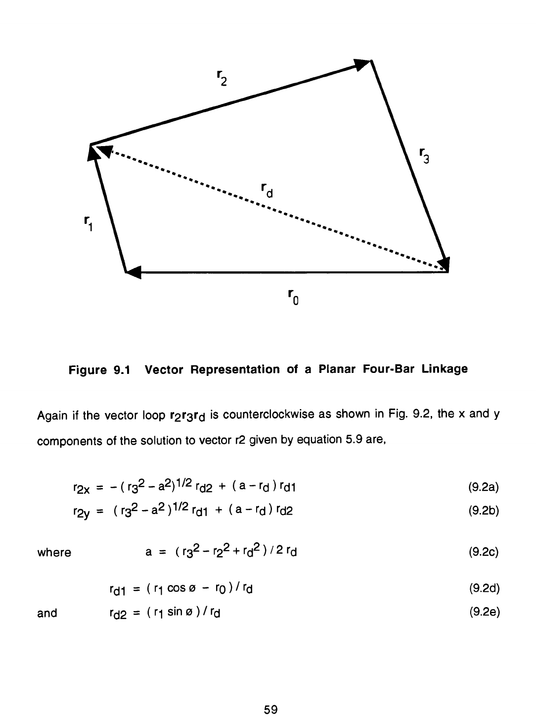
Figure
9.1
Vector
Representation
of
a
Planar
Four-Bar
Linkage
Again
if
the
vector
loop
r2r3rd
is
counterclockwise
as
shown
in
Fig.
9.2,
the
x
and
y
components
of
the
solution
to
vector
r2
given
by
equation
5.9
are,
"2x
=
-
(
r32
~
a2)1/2
rd2
+
(
a
"
rd
)
rd1
r2y
=
(
r32
~
a2
)1/2
rd1
+
(
a
-
rd
)
rd2
where
a
=
(r32-r22
+
rd2)/2
rd
rdi
=
(
ri
cos
o
-
ro
)
/
rd
and
rd2
=
(
H
sin
0
)
/
rd
(9.2a)
(9.2b)
(9.2c)
(9.2d)
(9.2e)
59

Figure
9.2
Vector
Representation
of
a
Four-Bar
Linkage
(Alternative
Mode
of
Assembly)
9.
2.
1
Evans
Linkage
A
vector
representation
of
the
Evans
Linkage
is
shown
in
Fig.
9.3.
Evans
linkage
is
obtained
from
the
simple
four-bar
mechanism
by
simply
extending
the
coupler
(represented
by
the
vector
r2).
Therefore
the
formula
for
the
components
of
r'2
in
figure
can
be
derived
from
equations
9.1
as
r'2x
=
(r'2/r2)[(r32-a2)1/2rd2
+
(
a
-
rd
)
rd1
]
r'2y
=
(r'2/r2)[-(r32-a2)1/2rdi
+
(a-rd)rd2]
(9.3a)
(9.3b)
60

Figure
9.3
Vector
Representation
of
Evans
Linkage
From
which
the
coordinates
of
the
output
point
M
(x,y)
are
obtained
as
and
x
=
r'2x
+
ri
cos
0
y
=
r'2y
+
r1
sin
0
(9.4a)
(9.4b)
The
coupler
point
curve
for
Evans
linkage
is
obtained
by
substituting
the
value
of
0
from
0
to
360
in
small
increments
and
plotting
the
positions
of
the
coupler
point
successively.
Appendix
B
gives
the
the
computer
program
that
utilizes
this
algorithm
61

and
plots
the
output
curve
for
a
given
set
of
dimensions
of
the
links.
Appendix
A
gives
some
samples
of
plots
thus
obtained.
9.
2.
2
Chebyshev
Linkage
A
Chebyshev
linkage
is
a
crank-rocker
mechanism
in
which
the
coupler
rotates
through
360.
A
schematic
representation
of
the
Chebyshev's
mechanism
is
shown
in
Fig.
9.4.
Since
the
output
point
M
may
lie
anywhere
on
the
coupler,
the
value
of
the
Figure
9.4
Vector
Representation
of
Chebyshev
Linkage
62

vector
r'2
is
unchanged
from
that
of
r2
given
by
equation
9.11
except
for
its
magnitude.
The
components
of
vector
r'2
is
calculated
as
follows:
r
2x
=
(
r'2
/
r2
)
[ (
r32
-
a2)1/2
rd2
+
(
a
-
rd
)
rd
]
(9.5a)
r'2y
=
(
r'2
/
r2
)
[
-
(
r32
-
a2
)1/2
rd1
+
(
a
-
rd
)
rd2
]
(9.5b)
The
position
vector
of
the
point
can
be
obtained
by
the
vector
addition
of
vectors
ri
and
r'2-
x
=
r'2x
+
r-|
cos
0
(9.6a)
and
y
=
r"2y
+
r-\
sin
0
(9.6b)
The
output
curve
can
be
obtained
by
by
finding
the
position
for
small
increments
of
0
between
0max
and
0mjn
using.
And
in
the
same
way
the
positions
are
calculated
for
the
second
half
rotation
of
the
coupler
using,
r'2x
=
(
r'2
/
r2
)
[
-
(
r32
-
a2)1/2
rd2
+
(
a
-
rd
)
rd1
]
(9.7a)
r
2y
=
(
r'2
/
r2
)
[
(
r32
-
a2
)1'2
rd1
+
(
a
-
rd
)
rd2
]
(9.7b)
Chapter
4
explains
these
limiting
angles
0max
and
0min-
and
how
to
calculate
them.
A
computer
code
developed
using
the
above
algorithm
to
plot
the
coupler
point
curves
for
Chebyshev
Linkage
is
given
in
Appendix
B
and
Appendix
A
contains
the
plots
obtained
from
the
program.
9.
2.
3
Watts
Linkage
Although
Watts
linkage
looks
similar
to
Chebyshev
Linkage,
it
differs
from
it
in
the
sense
that
none
of
the
links
rotates
through
360.
The
vector
representation
of
the
watts
linkage
is
shown
in
Fig.
9.5.
The
procedure
for
generation
of
the
coupler
curve
63

Figure
9.5
Vector
Representation
of
Watts
Linkage
for
Watts
linkage
is
done
the
same
way
as
that
of
Chebvshev's
except
that
its
limiting
angles
are
different.
These
limiting
angles
are
explained
in
Chapter
4.
For
the
first
half
of
the
coupler
curve,
the
positions
for
everv
small
increments
of
angles
between
0max
and
omjn
are
calculated
using,
r'2x
=
(
r*2
/
r2
)
[
(
r32
-
a2)1/2
rd2
+
(
a
-
rd
)
rd1
]
r'2y
=
(r,2/r2)[-(r32-a2)1/2rdi
+
(a-rd)rd2]
(9.8a)
(9.8b)
64

And
for
the
second
half
using
r
2x
=
(
r'2
/
r2
)
[
-
(
r32
-
a2)1/2
rd2
+
(
a
-
rd
)
rd1
]
(9.9a)
r'2y
=
(
r'2
/
r2
)
[
(
r32
-
a2
)1/2
rd1
+
(
a
-
rd
)
rd2
]
(9.9b)
where
a,
rdi
and
rd2
are
calculated
as
before
and
the
position
vector
of
the
point
can
be
obtained
by
the
vector
addition
of
vectors
r<\
and
r^.
x
=
r'2X
+
M
coso
(9.10a)
and
y
=
r*2y
+
r-\
sin
0
(9.10b)
Appendix
A
contains
some
samples
of
the
plots
generated
using
computers
and
the
codes
required
to
generate
those
plots
can
be
found
in
Appendix
B.
9.
2.
4
Roberts
Linkage
The
vector
representation
of
a
symmetrical
Roberts
Linkage
is
shown
in
Fig.
9.6.
As
we
have
seen
already
the
x
and
y
components
of
the
vector
r2
can
be
calculated
from
equations
9.1a
through
9.1e.
The
coordinates
(x-|
,y-|
)
and
(x2,y2)
are
calculated
as
follows,
x-|
=
rt
coso
(9.11a)
y-l
=
ri
sino
(9.11b)
x2
=
xi+r2x
(9.12a)
y2
=
yi+r2y
(9.12b)
65

Figure
9.6
Vector
Layout
of
Roberts
Linkage
To
find
the
coordinates
of
the
point
M(x,y),
from
Figure
9.6,
by
the
cosine
law,
r2
_
r22
+
r2
_
2
r
r2
cos
6
=>
6
=
cos~1
[
r2
/
2
r
]
(9.13)
and
the
angle
\\r
=
sin"1
[
(
yi
-
y2
)
/
r2
]
(9.14)
66

Finally
the
coordinates
of
the
output
point
M
are
obtained
by,
x
=
xi
+
rcos
(6
+
\|0
(9.15a)
and
y
=
y-j
-rsin
(G
+
v)
(9.15b)
These
coordinates
of
the
coupler
point
can
be
found
for
small
intervals
of
0
between
0mjn
and
0max
(see
Chapter
4
on
how
to
calculate
them).
The
computer
generated
plots
and
codes
for
Roberts
Linkage
are
given
Appendix
A
and
Appendix
B
respectively.
67

10.
SYNTHESIS
PROCEDURE
FOR
DESIGNING
A
FOUR-BAR
LINKAGE
TO
GENERATE
STRAIGHT
LINE
COUPLER
CURVE
In
the
linkages
studied,
conditions
have
been
developed
for
a
mechanism
to
generate
a
straight
line
and
numerical
and
geometrical
methods
to
study
these
outputs
are
also
discussed
in
detail.
However
it
is
a
different
task
to
start
with
a
required
straight
line
motion
and
to
try
to
proportion
a
mechanism
to
produce
this
motion.
This
procedure
is
known
as
the
synthesis
of
mechanisms.
In
the
application
of
synthesis
to
design
of
a
mechanism
,
the
problem
divides
itself
into
two
parts
(a)
the
type
of
mechanism
to
be
used,
(b)
the
proportions
and
lengths
of
the
links
necessary.
Analysis,
as
applied
to
mechanisms,
implies
that
given
the
dimensions
of
a
linkage
it
is
required
to
find
its
motion
characteristics.
Synthesis
will
be
the
exact
opposite;
the
motion
characteristics
are
specified
and
it
is
needed
to
find
the
linkage
that
will
produce
the
specified
motion.
These
design
of
linkages
for
specific
applications
relies
heavily
on
human
judgment
and
ingenuity.
This
design
process
may
be
illustrated
by
the
flow
chart
given
in
Figure
10.1.
This
process
of
human
interaction
includes
creativity
and
possibly
mathematical
analysis
and
computation
for
which
the
dimensional
requirements
that
have
been
derived
so
far
and
the
computer
codes
that
have
been
developed
will
be
of
immense
help.
While
it
is
unlikely
that
human
creativity
can
be
completely
replaced,
these
tools
and
knowledge
can
be
employed
to
relieve
the
designer
of
many
of
the
routine
processes
that
would
be
otherwise
necessary.
This
chapter
gives
the
designer
a
synthesis
procedure
in
order
to
help
him/her
to
select
and
design
a
four-bar
linkage
that
will
meet
the
design
criteria
and
will
provide
means
to
check
its
performance,
and
save
some
laborious
trial
and
error
processes.
68

Design
Situation
Select
Performance
Specifications
(P.
S.)
Reexamine
Design
Situation
Select
Design
Configuration
Set
Dimensions
Analyze
Proposed
Design
Yes
Acceptable
Design
Figure
10.1
The
Design
Process
69

10.
1
Kinematic
Synthesis
As
it
was
said
earlier
the
synthesis
of
a
four-bar
linkage
requires
the
designer
to
reach
decisions
on
(1)
the
form
or
type
of
mechanism,
(2)
the
proportions
(lengths)
of
the
links
necessary
to
accomplish
the
specified
motion
transformation.
The
first
phase
is
called
the type
synthesis.
Here
the
choice
of
the
linkage
mechanism
is
determined.
The
other
phase
is
dimensional
synthesis,
presents
challenging
problems,
to
which
the
greater
part
of
this
work
is
addressed.
10.
1.
1
Type
synthesis
The
selection
of
the
type
of
four-bar
linkage
needed
to
accomplish
a
purpose
depends
to
a
great
extent
on
consideration
of
usage,
the
coordination
of
input
and
output
and
availability.
If
the
mode
of
input
is
a
motor,
which
often
is,
the
choice
of
a
crank
rocker
mechanism
(such
as
Evans
linkage
and
Chebyshev
linkage)
would
be
appropriate,
since
in
this
type
of
mechanism
the
input
link
is
capable
of
complete
revolutions.
On
the
other
hand,
if
the
input
is
from
a
rocker
as
in
steam
engine
configuration,
Watts
linkage
or
Roberts
linkage
could
be
useful.
As
the
coupler
curve
plots
in
Appendix
A
show
that
the
coupler
curve
for
Watts
linkage
has
a
double
point
on
its
output,
it
could
be
used
as
the
return
mechanism
as
well.
With
so
many
factors,
there
can
be
no
scheme
whereby
a
mechanism
may
be
uniquely
determined
on
naming
desired
motion
specifications.
It
will
be
necessary
to
consider
a
line-up
of
possible
combinations
that
could
do
the
job,
from
which
the
"best
one"
for
the
particular
application
in
view
is
chosen.
10.
1.
2
Dimensional
Synthesis
By
dimensional
synthesis,
it
is
meant
determination
of
the
dimensions
of
parts
necessary
to
create
a
mechanism
that
will
effect
a
desired
motion
transformation.
In
70

considering
the
dimensional
synthesis,
it
recognized
that
it
has
two
aspects,
called
approximate
and
exact.
For
approximate
synthesis,
Chapter
8
provides
the
dimensional
conditions
for
a
four-bar
linkage
to
produce
a
straight
line
coupler
curve
as
follows:
0
B
Figure
10.2
Evans
Linkage
for
Symmetrical
Coupler
Curves
For
a
symmetrical
Evans
Linkage
shown
in
Figure
10.2,
(1+p)3/2
a
=
(10.1)
where
the
length
of
the
crank
is
considered
as
unity.
The
above
condition
is
true
to
the
dimensional
ratio
of
the
links.
This
means
any
multiple
of
these
dimensions
will
still
generate
a
straight
line.
It
can
be
seen
from
the
straight
line
plots
given
in
Appendix
A,
that
the
range
x
to
y
ration
decreases
as
p
increases.
The
designer
may
choose
a
p
value
that
suits
his
design
and
performance
restrictions.
71

Figure
10.3
A
Symmetrical
Chebyshev
Linkage
In
case
of
a
symmetrical
Chebyshev
linkage
as
the
one
in
Figure
10.3,
(
1
+
p
)3/2
r
=
(10.2)
2
here
the
length
of
the
coupler
which
can
rotate
completely
is
considered
as
one.
As
in
Evans
Linkage,
here
any
multiple
of
these
dimensions
will
produce a
straight
line
coupler
curve.
The
value
of
p
is
chosen
to
suit
the
needs
then
other
dimensions
are
determined
as
required
by
the
condition
10.2.
Geometric
methods
can
furnish,
with
superb
accuracy,
quick
and
dependable
solution
to
the
problem
of
exact
synthesis.
Chapters
9
is
dedicated
to
this
method
and
computer
codes
are
given
in
Appendix
B
that
are
created
to
provide
the
designer
the
graphical
means.
They
give
direct
feeling
for
mechanical
details
which
will
be
very
important
in
reducing
a
given
solution
to
hardware
and
which
may
be
obtained
directly
on
the
drawing
board
without
making
use
of
sometimes
unfamiliar
or
unavailable
analytical
techniques.
72

11.
CONCLUSION
The
objective
of
this
work
is
to
aid
a
designer
with
tools
and
knowledge
to
design
a
four-bar
mechanism
to
produce
a
straight
line
coupler
curve
that
would
meet
his/her
design
criteria.
In
this
work,
mechanisms
and
in
particular
four
bar
linkages
have
been
studied
and
their
components
and
classifications
have
been
discussed.
Four
special
four-linkages
that
are
capable
of
producing
a
straight
line
output
are
introduced
and
their
mobilities
have
been
explained
in
detail.
The
two
conditions
that
are
required
for
a
four-bar
mechanism
to
deliver
a
symmetrical
output
have
been
provided
along
with
their
proofs.
Two
crank
rocker
mechanisms
that
generate
straight
line
coupler
curve
have
been
analyzed
and
the
dimensional
requirements
in
order
for
them
to
generate
straight
lines
have
been
derived.
Position
analyses
of
all
the
links
in
a
four-bar
mechanism
have
been
done
using
vector
algebra
and
based
on
this,
separate
algorithms
to
numerically
generate
the
coupler
curves
have
been
arrived
at.
Computer
codes
and
the
plots
thus
obtained
are
added
in
appendices.
Finally,
synthesis
procedure
for
the
designer
to
design
a
mechanism
that
would
meet
his/her
needs
and
ways
to
make
finer
adjustments
to
meet
the
performance
criteria
are
provided.
It
has
thus
been
shown
that
it
is
possible
to
synthesize
a
four-bar
mechanism
analytically
that
could
generate
a
straight
line
as
part
of
its
coupler
curve.
This
work
73

will
help
the
designer
to
synthesize
analytically,
a
four-bar
mechanism
with
proper
selection
of
dimensions
thereby
saving
the
laborious
task
of
choosing,
by
trial
and
error,
a
mechanism
that
had
already
been
designed
which
would
rarely
coincide
the
requirements.
With
the
help
of
the
analytical
tools
presented
the
designer
could
also
make
finer
modifications
to
the
design
to
meet
exact
design
requirements.
Finally,
to
examine
the
output
of
the
mechanism
designed
the
graphical
methods
presented
would
be
an
excellent
tool.
74

References
1.
Hartenberg,
R.
S.
and
J.
Denavit,
Kinematic
Synthesis
of
Linkages.
New
York.
McGraw-Hill
Book
Company,
1964.
2.
Wilson,
C.
E.,
Sadler,
J.
P.
and
Michels,
W.
J.,
Kinematics
and
Dynamics
of
Machinery.
Harper
&
Row
Publishers,
New
York,
1983.
3.
Mabie,
H.
H.
and
Ocvirk,
F.
W,
Mechanisms
and
Dynamics
of
Machinery.
Third
Edition.
John
Wiley
&
Sons,
1975.
4.
Tao,
D.
C,
Applied
Linkage
Synthesis. Addison
-
Wesley
Publishing
Company,
lnc.1964.
5.
Lent,
D.,
Analysis
and
Design
of
Mechanisms.
Second
Edition.
Prentice-Hall,
Inc.,
New
Jersey,
1970.
6.
Vallence,
A.
and
Farris,
M.
E.,
Principles
of
Mechanism.
The
Macmillan
Company.
New
York,
1
933.
7.
S.
Molian,
The
Design
of
Cam
Mechanisms
and
Linkages.
American
Elsevier
Publishing
Company,
Inc.,
New
York,
1968.
8.
N.
Berzak,
Direct
Derivation
of
the
Symmetrical
Coupler
Curves
of
the
Planar
Four-Bar
Linkage.
75

9.
N.
Berzak,
Symmetrical
Coupler
Curves
from
Symmetrical
Four-Bar
Mechanisms.
10.
M.
A.
Chase,
Vector
Analysis
of
Linkages,
Transactions
of
American
Society
of
Mechanical
Engineers,
Journal
of
Engineering
for
Industries.
Series
B55,
No.
3
(August
1963):
pages
289
-
297
11.
E.
A.
Dilksman,
A
Modified
Design
for
l-Type
Double-Cranks
to
Approximate
a
Straight
Line,
Transactions
of
the
ASME.
Vol.
110,
December
1988,
pages
446-451.
12.
J.
A.
Hrones
and
G.
L.
Nelson,
Analysis
of
Four-Bar
Linkage;
Its
Application
To
The
Synthesis
of
Mechanisms,
Wiley,
New
York,
1
951
.
76

AIPIPIMIM
/A
\?LYB
IF
ira\QOT
UM
y[p[LI^

k*a
.--^
Fig.
A.1
Evans
Linkage

p
=
2.00,
r
=
1
.00,
s
=
2.59,
a
=
2.59
k
is
kept
as
2.00
EVANS
LINKAGE
p
=
2.00,
r=1.00,
s
=
2.50,
a
=
2.50
k
is
kept
as
2.00
EVANS
LINKAGE

p
=
3.00,
r
=
1
.00,
s
=
4.00,
a
=
4.00
k
is
kept
as
2.00
EVANS
LINKAGE
p
=
3.00,
r
=
1
.00,
s
=
4.10,
a
=
4.10
k
is
kept
as
2.00
EVANS
LINKAGE

p
=
4.00,
r
=
1
.00,
s
=
5.59,
a
=
5.59
k
is
kept
as
2.00
EVANS
LINKAGE
p
=
4.00,
r
=
1
.00,
s
=
5.90,
a
=
5.90
k
is
kept
as
2.00
EVANS
LINKAGE

p
=
5.00,
r
=
1
.00,
s
=
7.35,
a
=
7.35
k
is
kept
as
2.00
EVANS
LINKAGE
p
=
5.00,
r
=
1
.00,
s
=
7.95,
a
=
7.95
k
is
kept
as
2.00
EVANS
LINKAGE

p
=
6.00,
r
=
1
.00,
s
=
9.26,
a
=
9.26
k
is
kept
as
2.00
EVANS
LINKAGE
p
=
6.00,
r=
1.00,
s=
10.20,
a=
10.20
k
is
kept
as
2.00
EVANS
LINKAGE

Figure
A.2
Chebyshev
Linkage

p
=
2.00,
r
=
2.59,
s
=
2.59,
a
=
1
.00
CHEBYSHEV
LINKAGE
p
=
2.00,
r
=
2.50,
s
=
2.50,
a
=
1
.00
CHEBYSHEV
LINKAGE

p
=
3.00,
r
=
4.00,
s
=
4.00,
a
=
1
.00
CHEBYSHEV
LINKAGE
=
3.00,
r
=
4.10,
s
=
4.10,
a
=
1
.00
CHEBYSHEV
LINKAGE

p
=
4.00,
r
=
5.59,
s
=
5.59,
a
=
1
.00
CHEBYSHEV
LINKAGE
p
=
4.00,
r
=
5.90,
s
=
5.90,
a
=
1
.00
CHEBYSHEV
LINKAGE

p
=
5.00,
r
=
7.35,
s
=
7.35,
a
=
1
.00
CHEBYSHEV
LINKAGE
p
=
5.00,
r
=
7.95,
s
=
7.95,
a
=
1
.00
CHEBYSHEV
LINKAGE

p
=
6.00,
r
=
9.26,
s
=
9.26,
a
=
1
.00
CHEBYSHEV
LINKAGE
p
=
6.00,
r
=
1
0.20,
s
=
1
0.20,
a
=
1
.00
CHEBYSHEV
LINKAGE

"^-.
M
"*
Figure
A.3
Watts
Linkage

p
=
2.00,
r
=
1
.00,
s
=
1
.00,
a
=
1
.00
WATTS
LINKAGE
=
4.00,
r
=
2.00,
s
=
2.00,
a
=
2.00
WATTS
LINKAGE

p
=
4.00,
r
=
2.00,
s
=
2.00,
a
=
1
.00
WATTS
LINKAGE
p
=
5.00,
r
=
2.00,
s
=
2.00,
a
=
2.00
WATTS
LINKAGE

p
=
5.00,
r
=
2.00,
s
=
2.00,
a
=
3.00
WATTS
LINKAGE
p
=
5.00,
r
=
2.00,
s
=
2.00,
a
=
4.00
WATTS
LINKAGE

p
=
6.00,
r
=
1
.00,
s
=
1
.00,
a
=
5.00
WATTS
LINKAGE
p
=
6.00,
r
=
2.00,
s
=
2.00,
a
=
5.00
WATTS
LINKAGE

p
=
6.00,
r
=
2.00,
s
=
2.00,
a
=
3.00
WATTS
LINKAGE
p
=
6.00,
r
=
3.00,
s
=
3.00,
a
=
3.00
WATTS
LINKAGE

p
=
6.00,
r
=
3.00,
s
=
3.00,
a
=
1
.00
WATTS
LINKAGE
p
=
6.00,
r
=
3.00,
s
=
3.00,
a
=
2.00
WATTS
LINKAGE

p
=
6.00,
r
=
3.00,
s
=
3.00,
a
=
4.00
WATTS
LINKAGE
p
=
6.00,
r
=
2.00,
s
=
2.00,
a
=
4.00
WATTS
LINKAGE

Figure
A.4
Roberts
Linkage

p
=
2.00,
r
=
2.00,
s
=
2.00,
a
=
1
.00
b
=
2.00
ROBERTS
LINKAGE
p
=
3.00,
r
=
2.00,
s
=
2.00,
a
=
1
.00
b
=
1
.00
ROBERTS
LINKAGE

p
=
3.00,
r
=
3.00,
s
=
3.00,
a
=
1
.00
b
=
1
.00
ROBERTS
LINKAGE
p
=
4.00,
r
=
3.00,
s
=
3.00,
a
=
1
.00
b
=
1
.00
ROBERTS
LINKAGE

p
=
4.00,
r
=
2.00,
s
=
2.00,
a
=
2.00
b
=
3.00
ROBERTS
LINKAGE
p
=
4.00,
r
=
3.00,
s
=
3.00,
a
=
2.00
b
=
3.00
ROBERTS
LINKAGE

&[P^IM0^
@I
?
KMIKATTI

Evans.
p
Page
1
Friday,
April
15,
1994
3:04:18
PM
program
Evans;
{A
program
that
plots
the
coupler
curve
for
any
Evans
Mechanism}
var
xl,
yl:
array
[0..
200]
of
real;
rO,
M,
r2,
r3,
k,
w:real;
x,
y,
xmax,
xmin,
ymax,
ymin,
range:
real;
i,
xpos,
ypos,
cenl,
cen2,
cen3:
integer;
crank:
boolean;
capl,
cap2,
cap3:
string;
data:
text;
window,
trect:
rect;
procedure
initialize (window:
rect);
{initializes
the
windows}
begin
setrect(window,
0,
20,
screenbits.bounds.right,
screenbits.bounds.bottom);
setdrawingrect(window);
showdrawing;
end
^initialize}
procedure
readdata
(var
rO,
r1, r2,
r3,
k:
real);
{reads
data}
begin
readln(data,
rO,
r1,
r2,
r3,
k);
end;{readdata}
procedure
verify
(var
crank:
boolean;
rO,
r1,
r2,
r3:
real);
{verifies
if
the
data
complies
to
be
a
crank
rocker
mechanism}
var
lmax,
It,
la,
lb:
real;
begin
if
(M
<
rO)
and
(r1
<
r2)
and
(M
<
r3)
then
crank
:=
true
else
crank
:=
false;
if
crank
then
begin
lmax
:=
rO;
if
(M
>
lmax)
then
lmax
:=
r1
;
if
(r2
>
lmax)
then
lmax
:=
r2;
if
(r3
>
lmax)
then
lmax
:=
r3;
if
(rO
+
M
+
r2
+
r3
-
2
*
(lmax
+
r1))
>
0
then
crank
:=
true
else
crank
:=
false;
end;{if}
end;{verify}

Evans.
p
Page
2
Friday,
April
15,
1994
3:04:18
PM
procedure
iteration
(var
x,
y:
real;
rO,
r1,
r2,
r3,
k,
w:
real);
var
rd,
rd1,
rd2,
a,
r2x,
r2y:
real;
begin
rd
:=
sqrt(sqr(rO)
+
sqr(r1)
-
2
*
rO
*
r1
*
cos(w));
rd1
:=
(r1
*
cos(w)
-
rO)
/
rd;
rd2
:=
M
*
sin(w)
/
rd;
a
:=
(sqr(r3)
-
sqr(r2)
+
sqr(rd))
/
(2
*
rd);
r2x
:=
k
*
(sqrt(sqr(r3)
-
sqr(a))
*
rd2
+
(a
-
rd)
*
rd1
);
r2y
:=
k
*
(-sqrt(sqr(r3)
-
sqr(a))
*
rd1
+
(a
-
rd)
*
rd2);
x
:=
r2x
+
r1
*
cos(w);
y
:=r2y
+
r1
*sin(w);
end;{iteration}
begin
{main
program}
initialize(window);
reset(data,
'data');
readdata(rt),
r1,
r2,
r3,
k);
verify(crank,
rO,
M,
r2,
r3);
if
crank
then
begin
fori
:=0to
180
do
begin
w
:=
i
*
0.034906585;
iteration(x,
y,
rO,
M,
r2, r3,
k,
w);
xl[i]
:=
x;
yl[i]
:=
y;
end;{for}
xmax
:=xl[1];
ymax
:=yl[1];
xmin
:=xl[1];
ymin
:=yl[1];
fori
:=
1
to
180
do
begin
if
xl[i]
>
xmax
then
xmax
:=
xl[i];
if
yl[i]
>
ymax
then
ymax
:=
yl[i];
if
xl[i]
<
xmin
then
xmin
:=
xl[i];
if
yl[i]
<
ymin
then
ymin
:=
yl[i];
clpU=
stringofCp
=
',
rO
:
1
:
2,
\
r
=
\
M
:
1
:2,
\
s-\
r3
:
1
:2,
\
a
=
\r2:1:2);
cap2
:=
Stringof('
k
is
kept
as
',
k
:
1
:
2);
cenl
:=
300
-
stringwidth(cap1
)
div
2;
cen2
:=
300
-
stringwidth(cap2)
div
2;
moveto(cen1,
300);
drawstring(capl);

Evans.
p
Page
3
Friday,
April
15,
1994
3:04:18
PM
moveto(cen2,
325);
drawstring(cap2);
cap3
:=
stringofCEVANS
LINKAGE');
cen3
:=
300
-
stringwidth(cap3)
div
2;
moveto(cen3,
400);
drawstring(cap3);
range
:=
xmax
-
xmin;
if
(ymax
-
ymin
>
range)
then
range
:=
ymax
-
ymin;
xpos
:=
175
+
round(250
*
(xl[0]
-
xmin)
/
range);
ypos
:=
225
-
round(250
*
(yl[0]
-
ymin)
/
range);
moveto(xpos,
ypos);
fori
:=
1
to
180
do
begin
xpos
:=
175
+
round(250
*
(xl[i]
-
xmin)
/
range);
ypos
:=
225
-
round(250
*
(yl[i]
-
ymin)
/
range);
lineto(xpos,
ypos);
end;{forj
end
else
begin
setrect(trect,
100,
125,
400,
175);
settextrect(trect);
showtext;
writeln;
writeln('Sorry!
This
is
not
a
crank
rocker
mechanism!!');
end;{else}
end.{evans}

Chebyshev.
p
Page
1
Tuesday,
March
22,
1994
8:55:11
PM
program
Chebyshev;
{A
program
that
plots
the
coupler
curve
for
any
Chebyshev
Mechanism}
var
xl,
yl:
array[1
..200]
of
real;
rO,
M,
r2,
r3,
w:
real;
x,
y,
xmax,
xmin,
ymax,
ymin,
range:
real;
i,
xpos,
ypos,
cenl,
cen2:
integer;
crank:
boolean;
capl,
cap2:
string;
data:
text;
window,
trect:
rect;
procedure
initialize
(window:
rect);
{initializes
the
windows}
begin
setrect(window,
0, 20,
screenbits.bounds.right,
screenbits.bounds.bottom);
setdrawingrect(window);
showdrawing;
end
^initialize}
procedure
readdata
(var
rO,
r1, r2,
r3:
real);
{reads
data}
begin
readln(data,
rO,
M,
r2,
r3);
end;{readdata}
procedure
verify
(var
crank:
boolean;
rO,
r1, r2,
r3:
real);
{verifies
if
the
data
complies
to
be
a
double
rocker
mechanism}
var
lmax,
It,
la,
lb:
real;
begin
if
(M
<
rO)
and
(r1
<
r2)
and
(M
<
r3)
then
crank
:=
true
else
crank
:=
false;
if
crank
then
begin
lmax
:=
rO;
if
(M
>
lmax)
then
lmax
:=
r1
;
if
(r2
>
lmax)
then
lmax
:=
r2;
if
(r3
>
lmax)
then
lmax
:=
r3;
if
(rO
+
M
+
r2
+
r3
-
2
*
(lmax
+
r1))
>
0
then
crank
:=
true
else
crank
:=
false;
end;{if}
end;{verify}

Chebyshev.
p
Page
2
Tuesday,
March
22,
1994
8:55:11
PM
procedure
iteration
(var
x,
y:
real;
rO,
r1,
r2,
r3,
w:
real);
var
rd,
rd1,rd2,
a,
r2x,
r2y:
real;
r,
x1,y1,x2,
y2,
t,
p:
real;
begin
rd
:=
sqrt(sqr(rO)
+
sqr(r1
)
-
2
*
rO
*
r1
*
cos(w));
rd1
:=
(r1
*
cos(w)
-
rO)
/
rd;
rd2
:=
M
*
sin(w)
/
rd;
a
:=
(sqr(r3)
-
sqr(r2)
+
sqr(rd))
/
(2
*
rd);
r2x
:=
sqrt(sqr(r3)
-
sqr(a))
*
rd2
+
(a
-
rd)
*
rd1
;
r2y
:=
-sqrt(sqr(r3)
-
sqr(a))
*
rd1
+
(a
-
rd)
*
rd2;
x1
:=
r2x
+
M
*
cos(w);
y1
:=r2y
+
M
*sin(w);
x2
:=
(M
/
2)
*
cos(w);
y2:=(M
/2)*sin(w);
x
:=
x2
-
rO;
y
:=
y2;
r
:=
sqrt(sqr(x)
+
sqr(y));
t
:=
arcsin(y2
/
r);
p
:=arcsin((r0-x1)/r3);
x
:=
r
*
sin(t
+
p);
y
:=
r
*
cos(t
+
p);
end,
{iteration}
begin
{Main
Program}
initialize(window);
reset
(data,
'data');
readdata(rt),
ri,
r2,
r3);
verify(crank,
rO,
M
,
r2,
r3);
if
crank
then
begin
fori
:=
1
to
181
do
begin
w
:=
i
*
0.034906585;
iteration(x,
y,
rO,
M,
r2,
r3,
w);
xl[i]
:=
x;
yl[i]
:=
y;
end;{for}
xmax
:=xl[1];
ymax
:=yl[1];
xmin
:=xl[1];
ymin
:=yl[1];
fori
:=2to
181
do
begin
if
xl[i]
>
xmax
then
xmax
:=
xl[i];
if
yl[i]
>
ymax
then
ymax
:=
yl[i];
if
xl[i]
<
xmin
then

Chebyshev.p
Pa9e
3
Tuesday,
March
22,
1994
8:55:11
PM
xmin
:=
xl[i];
if
yl[i]
<
ymin
then
ymin
:=
yl[i];
end;{for}
capl
:=
stringof('p
=
',
r3
:
1
:
2,
',
r
=
',
rO
:
1
:
2,
',
s
=
',
r2
:
1
:
2,
',
a
=
',
M
:
1
:
2);
cenl
:=
300
-
stringwidth(capl)
div
2;
moveto(cen1,
300);
drawstring(capl);
cap2
:=
stringof('CHEBYSHEV
LINKAGE');
cen2
:=
300
-
stringwidth(cap2)
div
2;
moveto(cen2,
350);
drawstring(cap2);
range
:=
xmax
-
xmin;
if
(ymax
-
ymin
>
range)
then
range
:=
ymax
-
ymin;
xpos
:=
175
+
round(250
*
(xl[1]
-
xmin)
/
range);
ypos
:=
225
-
round(250
*
(yl[1]
-
ymin)
/
range);
moveto(xpos,
ypos);
fori
:=2to
181
do
begin
xpos
:=
175
+
round(250
*
(xl[i]
-
xmin)
/
range);
ypos
:=
225
-
round(250
*
(yl[i]
-
ymin)
/
range);
lineto(xpos,
ypos);
end;{forj
end
else
begin
setrect(trect,
100,
125,
400,
175);
settextrect(trect);
showtext;
writeln;
writelnj'Sorry!
This
is
not
a
double
rocker
mechanism!!');
end;{else}
end.{evans}

Watts.
p
Page
1
Tuesday,
March
22,
1994
9:04:27
PM
program
Watts;
var
xl,
yl:
array[1..200]
of
real;
rO,
M,
r2,
r3,
w,
d,
x,
y:
real;
wmax,
wmin,
xmax,
ymax,
xmin,
ymin,
range:
real;
i,
xpos,
ypos,
cenl
,
cen2:
integer;
crank:
boolean;
capl,
cap2:
string;
data:
text;
window,
trect:
rect;
procedure
initialize
(window:
rect);
begin
setrect(window,
0,
20,
screenbits.bounds.right,
screenbits.bounds.bottom);
setdrawingrect(window);
showdrawing;
end
^initialize}
procedure
readdata
(var
rO,
r1,
r2,
r3:
real);
begin
readln(data,
rO,
M,
r2,
r3);
end;{readdata}
procedure
verify
(var
crank:
boolean;
rO,
r1,
r2,
r3:
real);
begin
if
(M
+
r2
+
r3)
>
rO
then
crank
:=
true
else
crank
:=
false;
if
(rO
+
r2
+
r3)
>
M
then
crank
:=
true
else
crank
:=
false;
if
(rO
+
M
+
r3)
>
r2
then
crank
:=
true
else
crank
:=
false;
if
(rO
+
M
+
r2)
>
r3
then
crank
:=
true
else
crank
:=
false;
end;{verify}
procedure
iterationl
(var
x,
y:
real;
rO,
r1,
r2,
r3,
w:
real);
var
rd,
rd1,
rd2,
a,
r2x,
r2y:
real;
begin
rd
:=
sqrt(sqr(rO)
+
sqr(r1
)
-
2
*
rO
*
M
*
cos(w));

Watts.
p
Page
2
Tuesday,
March
22,
1994
9:04:27
PM
rd1
:=
(r1
*
cos(w)
-
rO)
/
rd;
rd2
:=
M
*
sin(w)
/
rd;
a
:=
(sqr(r3)
-
sqr(r2)
+
sqr(rd))
/
(2
*
rd);
r2x
:=
sqrt(sqr(r3)
-
sqr(a))
*
rd2
+
(a
-
rd)
*
rd1
;
r2y
:=
-sqrt(sqr(r3)
-
sqr(a))
*
rd1
+
(a
-
rd)
*
rd2;
x
:=(r2x/2)
+
M
*cos(w);
y
:=
(r2y
/
2)
+
M
*sin(w);
end
^iteration}
procedure
iteration2
(var
x,
y:
real;
rO,
r1,
r2,
r3,
w:
real);
var
rd,
rd1, rd2,
a,
r2x,
r2y:
real;
begin
rd
:=
sqrt(sqr(rO)
+
sqr(r1
)
-
2
*
rO
*
r1
*
cos(w));
rd1
:=
(r1
*
cos(w)
-
rO)
/
rd;
rd2
:=
M
*
sin(w)
/
rd;
a
:=
(sqr(r3)
-
sqr(r2)
+
sqr(rd))
/
(2
*
rd);
r2x
:=
-sqrt(sqr(r3)
-
sqr(a))
*
rd2
+
(a
-
rd)
*
rd1
;
r2y
:=
sqrt(sqr(r3)
-
sqr(a))
*
rd1
+
(a
-
rd)
*
rd2;
x
:=
(r2x
/
2)
+
r1
*
cos(w);
y
:=(r2y/2)
+
M
*sin(w);
end;{iteration}
begin
initialize(window);
reset(data,
'data');
readdata(rt),
M,
r2,
r3);
verify(crank,
rO,
M,
r2,
r3);
wmin
:=
-arccos((sqr(rO)
+
sqr(r1
)
-
sqr(r3
+
r2))
/
(2
*
rO
*
r1
))
+
0.0000001
;
wmax
:=
arccos((sqr(rO)
+
sqr(r1)
-
sqr(r3
+
r2))
/
(2
*
rO
*
r1))
-
0.0000001
;
if
crank
then
begin
d
:=
(wmax
-
wmin)
/
90;
for
i
:=
1
to
91
do
begin
w
:=
wmin
+
(i
-
1)
*d;
iteration1(x,
y,
rO,
M,
r2,
r3,
w);
xl[i]
:=
x;
yl[i]
:=
y;
end;{for}
fori
:=92to
182
do
begin
w
:=wmin
+
(182-
i)
*d;
iteration2(x,
y,
rO,
r1,
r2,
r3,
w);
xl[i]
:=
x;
yl[i]
:=
y;
end;{for}
xmax
:=xl[1];
ymax
:=yl[1];

Watts.
p
Page
3
Tuesday,
March
22,
1994
9:04:27
PM
xmin
:=xl[1];
ymin
:=yl[1];
fori
:=2to
182
do
begin
if
xl[i]
>
xmax
then
xmax
:=
xl[i];
if
yl[i]
>
ymax
then
ymax
:=
yl[i];
if
xl[i]
<
xmin
then
xmin
:=
xl[i];
if
yl[i]
<
ymin
then
ymin
:=
yl[i];
end;{for}
range
:=
xmax
-
xmin;
if
(ymax
-
ymin)
>
range
then
range
:=
ymax
-ymin;
capl
:=
stringof('p
=
',
rO
:
1
:
2,
',
r
=
',
r1
:
1
:
2,
',
s
=
',
r3
:
1
:
2,
',
a
=
',
r2
:
1
:
2);
cap2
:=
Stringof('WATTS
LINKAGE');
cenl
:=
300
-
stringwidth(cap1
)
div
2;
cen2
:=
300
-
stringwidth(cap2)
div
2;
moveto(cen1,
300);
drawstring(capl);
moveto(cen2,
350);
drawstring(cap2);
xpos
:=
175
+
round(250
*
(xl[1]
-
xmin)
/
range);
ypos
:=
225
-
round(250
*
(yl[1]
-
ymin)
/
range);
moveto(xpos,
ypos);
fori
:=2to
182
do
begin
xpos
:=
175
+
round(250
*
(xl[i]
-
xmin)
/
range);
ypos
:=
225
-
round(250
*
(yl[i]
-
ymin)
/
range);
lineto(xpos,
ypos);
end;{forj
xpos
:=
175
+
round(250
*
(xl[1]
-
xmin)
/
range);
ypos
:=
225
-
round(250
*
(yl[1]
-
ymin)
/
range);
lineto(xpos,
ypos);
end{if
crank}
else
begin
setrect(trect,
100,
125,
320,
175);
settextrect(trect);
showtext;
writeln;
writeln('Uh-huh!
This
is
not
gonna
work!!');
end;{else}
end.{watts}

Roberts.p
Page
1
Tuesday,
March
22,
1994
9:09:51
PM
program
Roberts;
var
xl,
yl:
array[1..200]
of
real;
rO,
M,
r2,
r3,
r,
t,
w,
d,
x,
y:
real;
wmin,
wmax,
xmax,
xmin,
ymax,
ymin,
range:
real;
i,
xpos,
ypos,
cenl
,
cen2,
cen3:
integer;
crank:
boolean;
capl,
cap2,
cap3:
string;
data:
text;
window,
trect:
rect;
procedure
initialize
(window:
rect);
begin
setrect(window,
0,
20,
screenbits.bounds.
right,
screenbits.bounds.bottom);
setdrawingrect(window);
showdrawing;
end
^initialize}
procedure
readdata
(var
rO,
r1, r2,
r3,
r:
real);
begin
readln(data,
rO,
r1,
r2,
r3,
r);
end;{readdata}
procedure
verify
(var
crank:
boolean;
rO,
r1,
r2,
r3:
real);
var
lmax,
It,
la,
lb:
real;
begin
if
(rO
>
r1)
and
(rO
>
r2)
and
(rO
>
r3)
then
crank
:=
true
else
crank
:=
true;
if
crank
then
if
(r1
+
r2
+
r3)
>
rO
then
crank
:=
true
else
crank
:=
false;
end;{verify}
procedure
iteration
(var
x,
y:
real;
rO,
r1,
r2,
r3,
r,
w:
real);
var
rd,
rd1
,
rd2,
a,
r2x,
r2y,
x1
,
y1
,
x2,
y2,
p:
real;
begin
rd
:=
sqrt(sqr(rO)
+
sqr(r1
)
-
2
*
rO
*
M
*
cos(w));
rd1
:=
(r1
*
cos(w)
-
rO)
/
rd;
rd2
:=
r1
*
sin(w)
/
rd;
a
:=
(sqr(r3)
-
sqr(r2)
+
sqr(rd))
/
(2
*
rd);
r2x
:=
sqrt(sqr(r3)
-
sqr(a))
*
rd2
+
(a
-
rd)
*
rd1
;
r2y
:=
-sqrt(sqr(r3)
-
sqr(a))
*
rd1
+
(a
-
rd)
*
rd2;

Roberts.p
Page
2
Tuesday,
March
22,
1994
9:09:51
PM
x1
:=
M
*
cos(w);
y1
:=M
*sin(w);
x2
:=
r2x
+
x1
;
y2
:=
r2y
+
y1
;
p
:=arcsin((y2-y1)/r2);
t
:=
arccos(r2
/
(2
*
r));
x
:=
x1
+
r
*
cos(p
-
1);
y:=y1
+r*sin(p-t);
end;{iteration}
begin
initialize(window);
reset(data,
'data');
readdata(rt),
M,
r2,
r3,
r);
verify(crank,
rO,
M,
r2,
r3);
wmin
:=
arccos((sqr(rO)
+
sqr(r1
+
r2)
-
sqr(r3))
/
(2
*
rO
*
(r1
+
r2)))
+
0.0000001
;
wmax
:=
arccos((sqr(r0)
+
sqr(r1)
-
sqr(r3
+
r2))
/
(2
*
rO
*
r1))
-
0.0000001
;
if
crank
then
begin
d
:=
(wmax
-
wmin)
/
1
80;
fori
:=1
to
181
do
begin
w
:=
wmin
+
(i
-
1)
*d;
iteration(x,
y,
rO,
r1,
r2, r3,
r,
w);
xl[i]
:=
x;
yl[i]
:=
y;
end;{for}
xmax
:=xl[1];
ymax
:=yl[1];
xmin
:=xl[1];
ymin:=yl[1];
fori
:=2to
181
do
begin
if
xl[i]
>
xmax
then
xmax
:=
xl[i];
if
yl[i]
>
ymax
then
ymax
:=
yl[i];
if
xl[i]
<
xmin
then
xmin
:=
xl[i];
if
yl[i]
<
ymin
then
ymin
:=
yl[i];
end;{for}
capl
:=
stringof('p
=
',
rO
:
1
:
2,
',
r
=
',
r1
:
1
:
2,
',
s
=
',
r3
:
1
:
2,
',
a
=
',
r2
:
1
:
2);
cap2
:=
Stringof('b
=
',
r
:
1
:
2);
cenl
:=
300
-
stringwidth(capl)
div
2;
cen2
:=
300
-
stringwidth(cap2)
div
2;
moveto(cen1,
300);
drawstring(capl);
moveto(cen2,
325);

Roberts.p
Page
3
Tuesday,
March
22,
1994
9:09:51
PM
drawstring(cap2);
cap3
:=
stringof('ROBERTS
LINKAGE');
cen3
:=
300
-
stringwidth(cap3)
div
2;
moveto(cen3,
400);
drawstring(cap3);
range
:=
xmax
-
xmin;
if
(ymax
-
ymin
>
range)
then
range
:=
ymax
-
ymin;
xpos
:=
175
+
round(250
*
(xl[1]
-
xmin)
/
range);
ypos
:=
225
-
round(250
*
(yl[1]
-
ymin)
/
range);
moveto(xpos, ypos);
fori
:=
2
to
181
do
begin
xpos
:=
175
+
round(250
*
(xl[i]
-
xmin)
/
range);
ypos
:=
225
-
round(250
*
(yl[i]
-
ymin)
/
range);
lineto(xpos,
ypos);
end;{for}
end
{if
crank}
else
begin
setrect(trect,
100,
125,
400,
175);
settextrect(trect);
showtext;
writeln;
writeln('Uh-huh!
This
is
not
gonna
work!!');
end;{else}
end.{evans}
