Historical Monetary Policy Analysis
and the Taylor Rule
Athanasios Orphanides
∗
Board of Governors of the Federal Reserve System
June 2003
Abstract
This study examines the usefulness of the Taylor-rule framework as an organizing device
for describing the policy debate and evolution of monetary policy in the United States.
Monetary policy during the 1920s and since the 1951 Treasury-Federal Reserve Accord
can be broadly interpreted in terms of this framework with rather surprising consistency.
In broad terms, during these periods policy has been generally formulated in a forward-
looking manner with price stability and economic stability serving as implicit or explicit
guides. As early as the 1920s, measures of real economic activity relative to “normal” or
“potential” supply appear to have influenced policy analysis and deliberations. Confidence
in such measures as guides for activist monetary policy proved counterproductive at times,
resulting in excessive activism, such as during the Great Inflation and at the brink of the
Great Depression. Policy during the past two decades is broadly consistent with natural-
growth targeting variants of the Taylor rule that exhibit less activism.
JEL Classification System: E3, E5, B2
Correspondence: Federal Reserve Board, Washington, D.C. 20551, Tel.: (202) 452-2654, e-mail:
Athanasios.Orphanides@frb.gov.
∗
Prepared for the Carnegie-Rochester Conference on Public Policy on the 10th anniversary of the
Taylor rule, Pittsburgh, PA, November 22-23, 2002. I would like to thank Oldrich Dedek, Gregory
Hess, William Keech, David Lindsey, Bennett McCallum, Allan Meltzer, William Poole, Richard
Porter, Simon van Norden, Anna Schwartz, Jan Qvigstad, as well as participants at the conference
and at presentations at Harvard University, George Mason University, the Norges Bank Workshop
on Monetary Policy Rules in Inflation Targeting Regimes, and the 2003 meeting of the American
Economic Association for helpful discussions and comments. The opinions expressed are those of
the author and do not necessarily reflect views of the Board of Governors of the Federal Reserve
System.
1 Introduction
In the decade since John B. Taylor’s celebrated essay on “Discretion versus policy rules in
practice” was presented at the 39th Carnegie-Rochester Conference on Public Policy in the
Fall of 1992, his analysis has had considerable influence on the way monetary economists
and practitioners think about the policy debate. Taylor showed that actual monetary policy
in the United States could be usefully described in terms of a simple rule that appeared
promising on the basis of policy evaluation experiments. Most importantly, he described
the monetary policy process in terms of the short-term nominal interest rate that was close
to the actual decision making process, and described policy directly in terms of the two
major operational objectives of monetary policy, inflation and economic growth.
My aim in this study is to investigate the usefulness of the Taylor-rule framework as an
organizing device for describing the policy debate and evolution of monetary policy in the
United States. Key to this undertaking is the examination of interest rate policy decisions
linked directly to the Federal Reserve’s underlying policy objectives, as these may have
been understood over time. In the spirit of Friedman and Schwartz (1963), I rely heavily
on narrative descriptions of events and ideas, supplemented, as possible, with information
available to policy practitioners when policy was made. A major difference is my reliance
on the language of interest-rate-based policies, instead of the stock of money, and some of
the resulting analysis can be seen as a re-interpretation of earlier findings using the latter
language. The ultimate goal of this effort is to use the historical experience to draw lessons
about past policy successes and policy errors.
The theme that emerges from this examination is that Federal Reserve policies over
many periods, virtually since the founding of the institution, can be broadly interpreted in
terms of the Taylor-rule framework with surprising consistency. The Taylor rule serves as a
particularly good description of policy, however, both when subsequent economic outcomes
were exemplary as well as less than ideal. A recurrent source of errors has been misper-
ceptions of the state of the economy, the result of incorrect assessments of the economy’s
productive potential. This concept has appeared in policy discussions with different names
and in various contexts from the first years of operation of the System. It has often led
to false predictions of inflation or disinflation, prompting tightening or easing actions that
1

were only recognized as counterproductive long after the fact. This historical analysis sug-
gests that the Taylor rule appears to serve as a useful organizing device for interpreting
past policy decisions and mistakes, but adoption of the Taylor-rule framework for policy
analysis is not insurance that past policy mistakes would not have occured.
2 Two Interpretations of the Taylor Rule
In his original exposition of a rule-based framework for monetary policy analysis, Taylor
offered two interpretations of rules-based policy. The first concentrated on an example
presented with a precise algebraic formula. The second emphasized the broad characteristics
of policy rules, recognizing that, as with virtually any rule, implementation details should
be left to policymakers. Although the precise algebraic formula caught most of the attention
originally, my analysis suggests that the broader interpretation is of at least as much interest,
especially for historical analysis. In this section, I review the two interpretations, and relate
the framework to an alternative simple rule motivated by money growth targeting.
2.1 A Narrow Interpretation: The Classic Taylor Rule
The specific example that captivated so much attention was presented by Taylor as a “hy-
pothetical but representative policy rule” (1993, p. 214). In effect, this example was a
particular parameterization of a policy rule that had already been studied in detail by par-
ticipants of the Brookings project on policy regime evaluation reported in Bryant, Hooper
and Mann (1993), and also examined in another contribution to the Fall 1992 Carnegie-
Rochester conference by Henderson and McKibbin (1993).
1
The Brookings study examined
rules setting deviations of the short-term nominal interest, i, from a baseline path, i
∗
,in
proportion to deviations of a target variables z, from its target, z
∗
.
i − i
∗
= θ(z − z
∗
)(1)
Among the alternative target variables examined, the collective findings in the Brookings
study pointed to two as more likely to result in better economic performance. One of
1
The Brookings conference, which took place in March 1990, and to which both Taylor, and Henderson and
McKibbin contributed, appears to have had an influence on the contributions by Taylor and by Henderson
and McKibbin to the 1992 Carnegie-Rochester conference. Taylor’s contribution on nominal GNP targeting
at an earlier Carnegie-Rochester conference (Taylor 1985), offered an earlier related analysis of some of the
issues that also appeared in the later work.
2

these suggested targeting the sum of the price level p, and real output q—that is nominal
income, p + q (“nominal income targeting regime”). The other suggested targeting the sum
of inflation, π =∆p, and real output (“real-output-plus-inflation targeting regime”):
2
i − i
∗
= θ((π + q) − (π
∗
+ q
∗
)) (2)
Variations of this formulation, with differential responses to inflation and output:
i − i
∗
= θ
π
(π − π
∗
)+θ
q
(q − q
∗
)(3)
were also considered in some of the contributions to the Brookings study. In his parameteri-
zation, Taylor adopted the “real-output-plus-inflation” variant and set the baseline nominal
interest rate to equal the sum of the equilibrium or natural rate of interest, r
∗
, and inflation,
π. He employed an output gap measure obtained from a smooth trend, y = q − q
∗
,and
used the year-over-year rate of change of the output deflator to measure inflation. Setting
the inflation target and equilibrium real interest equal to two and the response parameter,
θ to one half, he arrived at what we now know as the classic Taylor rule:
i =2+π +
1
2
(π − 2) +
1
2
(q − q
∗
)(4)
Taylor noted that this parameterization appeared to fit Federal Reserve behavior well over
the previous several years and observed: “If the policy rule comes so close to describing
actual Federal Reserve behavior in recent years and if FOMC members believe that such
performance was good and should be replicated in the future even under a different set of
circumstances, then a policy rule could provide some guidance to future decisions.” (p. 208.)
2.2 Some Limitations
Some of the suggested attractive qualities of this rule, however, were promptly questioned.
As McCallum (1993) noted, Taylor’s formulation was not “operational.” It required in-
formation that the policymaker did not necessarily have at his disposal.
3
Crucially, this
formula requires policymakers to take a stand on and formulate policy on the basis of implicit
2
Unless otherwise noted, I use capital letters to denote levels and small letters (except for interest rates)
to denote respective logarithms. Throughout, I use log differences to approximate rates of change, scaled to
annual rates, in percent. Interest rates are in percent, annual rates.
3
McCallum was originally concerned with the timing of information on inflation and the output gap.
Orphanides (2001, 2003) later demonstrated that the informational problem was broader and quantitatively
severe in practice, especially regarding the measurement of the “output gap.”
3

assumptions regarding concepts such as the natural rate of interest and potential output
(or the related natural rate of unemployment or “NAIRU”), which are known to be notori-
ously unreliable as policy indicators.
4
Not all academic observers and policy practitioners
believe such concepts are either necessary or helpful for formulating policy. Policymakers,
in particular, might prefer to avoid the dogmatic reliance on natural-rate-gap-based policy
rules, such as Taylor’s classic formulation.
5
At the very least, these difficulties serve as an important reason for viewing this par-
ticular rule as a strategy that could only be implemented with a substantial element of
discretion. This point was emphasized by Chairman Greenspan in 1997:
As Taylor himself has pointed out, these types of formulations are at best “guide-
posts” to help central banks, not inflexible rules that eliminate discretion. One
reason is that their formulation depends on the values of certain key variables–
most crucially the equilibrium real federal funds rate and the production po-
tential of the economy. In practice these have been obtained by observation of
past macroeconomic behavior–either through informal inspection of the data, or
more formally as embedded in models. In that sense, like all rules, as I noted
earlier, they embody a forecast that the future will be like the past. Unfortu-
nately, however, history is not an infallible guide to the future, and the levels of
these two variables are currently under active debate.
In addition, the classic Taylor rule lacks an explicit role for forecasts and related judgments
about prospective economic developments. As noted by Meyer (2002):
Although the Taylor rule has been a useful benchmark for policymakers, my
experience during the last 5-1/2 years on the FOMC has been that considerations
that are not explicit in the Taylor rule have played an important role in policy
deliberations. In particular, forecasts clearly have played a powerful role in
shaping the response of monetary policy in a way not reflected in the simple
Taylor rule.
Indeed, forecasts of the economic outlook have always served an important role in monetary
policy decisions at the Federal Reserve, with rather similar justifications being provided for
4
Quantifications of this unreliability are presented in several recent studies, including Staiger, Stock and
Watson (1997), and Laubach (2001), for the natural rate of unemployment; Christiano and Fitzgerald (2001),
Orphanides and van Norden (2002), and van Norden (2002) for potential output; Laubach and Williams
(2001), for the natural rate of interest and Orphanides and Williams (2002), for the natural rates of interest
and unemployment.
5
The classic exposition of the dangers of such natural-rate-gap-based policies appears in Friedman’s 1967
AEA presidential address, (Friedman, 1968).
4

this practice over the decades. Consider, for instance, the following remarks by Chairman
Greenspan from 1999 and the remarks by Chairman Martin in 1965, both offered during
periods when monetary policy was in a tightening phase and inflation appeared to be the
predominant threat.
For monetary policy to foster maximum sustainable economic growth, it is use-
ful to preempt forces of imbalance before they threaten economic stability. But
this may not always be possible—the future at times can be too opaque to pen-
etrate. When we can be preemptive, we should be, because modest preemptive
actions can obviate more drastic actions at a later date that would destabilize
the economy. (Greenspan, 1999)
To me, the effective time to act against inflationary pressures is when they are
in the development stage—before they have become full-blown and the damage
has been done. Precautionary measures are more likely to be effective than
remedial action: the old proverb that an ounce of prevention is worth a pound
of cure applies to monetary policy as well as to anything else. (Martin, 1965)
More generally, preemption appeared to be a guiding principle of the Federal Reserve as
early as the founding of the System. As the Board explained in its First Annual Report
for 1914, which was published in January 1915: “[A reserve bank’s] duty is not to await
emergencies but by anticipation, to do what it can to prevent them.”
Given that Federal Reserve officials have always described the formulation of monetary
policy as a forward-looking process, policy rules failing to incorporate such information into
historical analyses of policy decisions could easily prove inadequate. A popular approach is
to modify Taylor’s classic formulation by replacing current and recent outcomes in rules of
the form (3) with forecasts of these variables.
6
Alternatively, as suggested by Taylor (1993),
policymakers could consult the forecast path of the federal funds rate obtained by projecting
rule (3) using forecasts of inflation and economic activity. Attempting to incorporate an
explicit role for forecasts in a monetary policy rule, however, must be seen in the context
of a broader interpretation of policy rules than the one embedded in Taylor’s classic rule
example. I turn to such a broad interpretation next.
6
Examples of such variants in policy evaluations and descriptive exercises include Batini and Haldane
(1999), Batini and Nelson (2000), Clarida, Gali and Gertler (1999, 2000), Levin, Wieland and Williams
(1999, 2003), Nessen (1999) and Orphanides (2001, 2002, 2003).
5
2.3 A Broad Interpretation
The broad interpretation of Taylor’s rule-based framework for monetary policy provides
a degree of flexibility that addresses some of the perceived limitations of the classic rule.
In describing this broad interpretation Taylor stressed that “a policy rule need not be a
mechanical formula,” (1993, p. 198). Rather, adopting a position closer to earlier in-
terpretations of policy rules such as in Samuelson (1951, 1967) and Tobin (1983), Taylor
emphasized the broader definition of a rule as a systematic policy program geared towards
the attainment of the fundamental policy objectives. In general terms, Taylor described the
fundamental features of the policy he was proposing by quoting a useful summary descrip-
tion from the 1990 Economic Report of the President, (which, as a member of the Council
that year, he had co-authored):
The Federal Reserve generally increases interest rates when inflationary pres-
sures appear to be rising and lowers interest rates when inflationary pressures
are abating and recession appears to be more of a threat. (Council of Economic
Advisers, 1990, p. 85).
As with the classic, narrow interpretation, the objectives of monetary policy are to dampen
business cycle fluctuations and maintain price stability. But unlike the narrow interpreta-
tion, policymakers are given more leeway in taking actions to achieve the desired effect. This
permits the use of sound judgment outside the scope of any fixed formula in formulating
policy and without restricting policymakers necessarily to a specific analytical framework.
Of course, this broad interpretation has the disadvantage of reduced precision—indeed
as a policy rule it must be seen as one whose implementation requires discretion. On the
other hand, this broad interpretation of Taylor’s rule-based policy presents some substantial
advantages as a descriptive device. It maintains a role for pre-emption and the use of
forecasts in setting policy, and it accommodates the exhibited policymakers’ preference
for adopting explicitly forward-looking policy guides. Equally important, Taylor’s broad
interpretation does not require policymakers to accept natural-rate-gap-based policy as their
guiding principle. By being more encompassing, the broad interpretation of the Taylor rule
arguably better captures the actual policy process over time.
This broad interpretation of Taylor’s framework, as opposed to the classic Taylor rule,
also relates more closely to the inflation targeting approach to policy, discussed in Bernanke
6
and Mishkin (1997), and Bernanke, Laubach, Mishkin and Posen (1998). Indeed, as
Bernanke and Mishkin stress, inflation targeting is a framework of “constrained discretion.”
The broader interpretation of Taylor’s policy framework places its emphasis on the
identification of the System’s operational objectives regarding price stability and economic
growth and asks that policymakers apply their collective judgment to adjust interest rates
so as to balance the perceived risks with regard to the outlook for the two objectives. In
this sense, the crucial element for interpreting historical monetary policy with the Taylor
rule rests on two elements: First, the extent to which the System has relied on short-term
interest rates as its primary policy instrument, which is widely accepted as a fairly accurate
description. Second, the evolution of the System’s operational objectives vis-a-vis price
stability and economic growth, as interpreted by policymakers over time for the conduct of
policy. As I illustrate next, policymaking in the System has broadly exhibited a remarkable
consistency in this regard as well. The System’s consistency with regard to these two key
elements of the Taylor-rule framework through time provides the strongest rationale for the
usefulness of the framework for interpreting historical monetary policy decisions.
2.4 Policy Objectives and Strategy Over Time
An appropriate starting point for examining the evolution of policy objectives and their
interpretation is to examine the current statutory objectives of the System, as reflected in
the November 16, 1977 amendment of Section 2A of the Federal Reserve Act. These are:
“maximum employment, stable prices, and moderate long-term interest rates.” A recent
operational interpretation can be found in the Committee’s January 19, 2000 statement
which introduced the practice of announcing: “the FOMC’s consensus about the balance
of risks to the attainment of its long-run goals of price stability and sustainable economic
growth.” Related interpretations of the dual objective of price stability and maximum
growth can be traced back to the legislative mandate of the Employment Act of 1946. As
an illustration, consider the following statement from a 1957 Congressional Hearing:
The objective of the System is always the same—to promote monetary and credit
conditions that will foster sustained economic growth together with stability in
the value of the dollar. (United States Congress, 1957, p. 1252.)
7
However, even before the 1946 Act, the Federal Reserve appeared to be interpreting its
“implicit” objectives in rather similar terms. The following statement from the Annual
Report for 1945 suggests a modern interpretation of both the goals of policy, as well as the
broad guiding principles for Taylor’s conduct of policy:
It is the Board’s belief that the implicit predominant purpose of Federal Reserve
policy is to contribute, insofar as the limitations of monetary and credit policy
permit, to an economic environment favorable to the highest possible degree of
sustained production and employment. Traditionally, this over-all policy has
been followed by easing credit conditions when deflationary factors prevailed
and, conversely, by restricting measures when inflationary forces threatened.
Indeed, as Chairman McCabe noted in 1949: “... for the entire period since 1935, Federal
Reserve credit policies have been altogether in conformity with the objectives stated in
the Employment Act of 1946. Review of a longer period would show that throughout
the System’s existence Federal Reserve objectives have been in harmony with these broad
purposes.” (Joint Committee on the Economic Report, 1949, p. 25-26.)
2.5 Monetary Growth Targeting in the Taylor Framework
The broad interpretation of the Taylor rule is also of interest because it permits investi-
gations of alternative specific policy rules that are consistent with the attainment of the
policy objectives of price stability and maximum sustainable growth.
One such example may be viewed as a reformulation of Friedman’s monetary growth
rule in terms of the family of policy rules investigated in the Brookings study. Recall that
one of the key advantages of Friedman’s money growth rule is that is stays clear of the
pitfalls known to plague the natural-rate-gap-based policy approach. In terms of rule (1),
a strategy that meets this criterion but maintains the spirit of the “nominal income” and
“real-output-plus-inflation” targeting regimes considered in the Brookings project, is to set
the growth (instead of the level) of nominal income, ∆(p+q)=π +∆q, as the target variable
z, and rely on the lagged value of the interest rate instrument as the baseline for policy
adjustments. The resulting rule becomes:
∆i = θ((π +∆q) − (π
∗
+∆q
∗
)) (5)
To see the relationship to money growth targeting recall that, given a monetary aggregate,
8

m, and its velocity, v, the equation of exchange implies:
∆m +∆v = π +∆q (6)
Allowing for adjustments in the change of equilibrium velocity and potential output growth,
a non-activist money growth rule with the objective of achieving an inflation target π
∗
sets:
7
∆m = π
∗
+∆q
∗
− ∆v
∗
(7)
or, after substituting the equation of exchange, stated in terms of velocity:
∆v − ∆v
∗
=(π − π
∗
)+(∆q − ∆q
∗
)(8)
To reformulate this strategy in terms of an interest rate rule, consider the simplest formu-
lation of money demand as a (log-) linear relationship between velocity deviations from its
equilibrium and the rate of interest. In difference form this is:
8
∆v − ∆v
∗
= a∆i + e (9)
where a>0ande summarizes short-run dynamics and money-demand fluctuations. Sub-
stituting (9) into (8) but without the term e—that is avoiding the short-run velocity fluctu-
ations which are the suggested principal drawback of money growth strategies that interest-
rate based strategies are designed to avoid—yields:
∆i = θ((π − π
∗
)+(∆q − ∆q
∗
)) (10)
where θ>0. As can be readily seen, this has exactly the same form as rule (5). More
generally, money growth rules that incorporate additional responses to inflation, real output
7
For example, Friedman’s famous 4% rule for the growth of M2 during the late 1960s and early 1970s,
corresponded to a zero inflation target with the assumptions that M2 velocity exhibited no trend and
potential output growth equaled 4% (the prevailing estimate at the time), or with the assumption of a
somewhat smaller estimate of potential output growth and a corresponding small downward trend in velocity.
8
This reformulation presupposes that interest rates are positive and not near the zero bound. If additional
monetary easing is required when the rate is at zero, it can be easily achieved by increasing the rate of money
growth further, but this easing is obviously not reflected in additional reductions in the interest rate policy
instrument. This break in the link between interest rates and easy money sometimes leads to the flawed
conclusion that no additional easing is possible at the zero bound. (Examples would be the experience during
the Great Depression and, more recently, in Japan. See Orphanides, 2003d, for details.) As Taylor stressed
at a 1995 Bank of Japan conference, the deflation experienced at the time in Japan “made an interest rate
rule unreliable, calling for greater emphasis on money supply rules.” (Taylor 1997, p. 36). Orphanides
and Wieland (2000) elaborate on this transition from Taylor-rule-based to money-based policies under these
circumstances. Using data from the Great Depression and recent Japanese experience, they also illustrate
how the simple velocity-interest rate relationship reflected in (9) breaks down at the zero bound.
9

growth or nominal output growth, such as rules in the spirit of Brunner, Cooper, Fischer,
McCallum and Meltzer, which can be written as:
9
∆m = π
∗
+∆q
∗
− ∆v
∗
− b
π
(π − π
∗
) − b
∆q
(∆q − ∆q
∗
) (11)
for b
π
,b
∆q
≥ 0 can be similarly reformulated as
∆i = θ
π
(π − π
∗
)+θ
∆q
(∆q − ∆q
∗
) (12)
for positive values of θ
π
and θ
∆q
. To differentiate these specific rules from Taylor’s classic
formulation, I will refer to them as natural-growth targeting rules to highlight that these
rules rely on estimates of the economy’s natural growth rate for guidance, responding to
perceived imbalances between the growth of aggregate demand and aggregate supply, and
not an output gap.
10
In words, these natural-growth targeting rules call for the Federal Reserve to raise
interest rates “when inflationary pressures appear to be rising” and lower rates “when
inflationary pressures are abating and recession appears to be more of a threat,” matching
quite closely Taylor’s verbal description of the broad guidelines for an interest-rate-based
rule described earlier. Indeed, Taylor himself stressed the broad relation of money growth
targeting rules and his interest-rate-based policy framework (1993, p. 209 and 1999, p. 322)
and also suggested “a policy rule where the growth rate of GDP rather than its level appears”
(1993, p. 208) as one of the examples of specific rules that Federal Reserve staff could
present to the FOMC as part of the policy decision process.
11
The reliance of information
regarding growth rates, as opposed to natural-rate gaps, is also not inconsistent with verbal
descriptions of policy considerations.
12
As with Taylor’s classic alternative, natural-growth
9
Brunner and Meltzer (1993), Cooper and Fischer (1972, 1974), Fischer and Cooper (1973), Meltzer
(1987), McCallum (1988, 1990, 2000).
10
Rules (10) and (12) also relate to price level targeting and to nominal income targeting rules, stated in
difference form. Letting n = π +∆q denote the growth of nominal income and n
∗
= π
∗
+∆q
∗
denote the
natural growth of nominal income, given the desired rate of inflation, the simplest form, (10), can be written
more simply as: ∆i = θ(n− n
∗
). Orphanides and Williams (2002) offer detailed econometric policy evaluation
comparisons of rules of the form (3) and (12) and an extensive bibliography of earlier studies examining
the relative merits of the level/difference elements of the two alternatives. See, in particular, Goodfriend
(1991), Levin et al (1999), Rotemberg and Woodford (1999), Sack and Wieland (2000), Williams (1999)
and Woodford (1999) for the role of interest smoothing and Leitemo and Lonning (2001), McCallum (2001),
Orphanides et al (2000), Woodford (2002), and Walsh (2003) for the role of output growth.
11
McCallum (2000) and Razzak (2003) also investigated the relation between money-growth and interest-
rate-based policy rules. A grandparent of such comparisons is the classic study by Poole (1970).
12
A recent example to this effect appeared in remarks by Chairman Greenspan articulating his concerns
10

targeting rules could be implemented based on either current data and recent realizations
of inflation and output growth, or based on the outlook of inflation and growth in the near
future.
3 Monetary Policy Since the Treasury-Federal Reserve Ac-
cord Through the Lens of a Taylor Rule
Figure 1 provides a summary overview of macroeconomic developments in the United States
since 1951—the year that marked the re-birth of the System following the subordination
of Federal Reserve policy to Treasury financing operations during World War II.
13
The top
panel shows the familiar path of inflation, measured as the rate of change of the output
(GDP) deflator over four quarters. The middle panel plots real output growth over four
quarters (solid line) as well as an estimate of the natural rate of growth of the economy over
time—the growth of potential output (dotted line). The bottom panel plots an estimate of
the output gap. All data in the figure are the most recently available estimates, as produced
by the Commerce Department for the GDP data and by the Congressional Budget Office
for potential output. As is well known, all of these series, but particularly the estimates
of potential output, are subject to revisions, redefinitions, rebenchmarks, remodeling and
so forth—an issue whose significance will become evident shortly. In this, and subsequent
figures, the vertical dotted lines represent business cycle peaks and troughs as dated by the
National Bureau of Economic Research (NBER). (The narrow spacing reflects peaks and
the wide spacing troughs, respectively. As of this writing, the date of the trough of the
recession that started in 2001 has not been announced.)
Historical policy evaluation is seen as an attempt to explain the interactions of policy
decision with subsequent economic outcomes, and to assess whether policy action or inaction
was appropriate in terms of its direction, timing and perhaps magnitude. The most precise
method for such evaluations requires the use of a model. Such evaluations, however, are
limited by and the results are conditioned upon the confidence with which we can hold
that the model serves as an adequate representation of reality for that purpose. Given our
about the economic outlook in January 2000, during a tightening policy phase: “It is this imbalance between
growth of supply and growth of demand that contains the potential seeds of rising inflationary and financial
pressures that could undermine the current expansion.”
13
Hetzel and Leach (2001) provide a fascinating narrative account of the events leading to the March 4,
1951 Accord.
11
severely limited knowledge of the workings of the economy, we can therefore never hope
to be able to evaluate specific actions with much accuracy, even in hindsight. We may,
however, succeed in pinpointing particular periods when better outcomes would appear to
have been likely, at least with the benefit of hindsight, had better policies been pursued.
For example, retrospectively, it is sometimes straightforward to identify periods when the
economy was overheated and inflation was deviating from price stability. Based on just
rudimentary knowledge of the monetary transmission mechanism and its lags, those are
periods before which tighter monetary policy would have been seen as more successful than
its actual path. Consider, for instance, the years surrounding 1955, 1965, 1978—to select
just an example from each of the first three decades shown. In each case, according to
the figure, output exceeded its potential, output growth exceeded the growth of potential
supply, and inflation worsened. In each case, if an outside observer to the System could have
rerun that particular episode in history (with the benefit of hindsight), tighter monetary
policy would have likely been suggested.
In general, for a suggested monetary policy framework to be seen as an improvement
over the arrangements that in fact were put in place over history, it must be the case that
the framework would have suggested a better policy, at least over some of these clearly
identifiable periods, and no worse policy at most other times. Accurate identification of
any suggested improvement, however, requires that policy rule prescriptions from a rule
under consideration be based on information available to policymakers when decisions are
made, as opposed to information that has become available ex post. This distinction is
of particular significance for natural-rate-gap-based policy rules as natural rate concepts
are particularly prone to revision on the basis of the subsequent evolution of the economy,
which is obviously unknown when policy decisions are made.
In this section, I conduct counterfactual analyses of the Taylor rule over the past half
century examining the performance of such strategies with the criteria outlined above. To
illustrate the dangers of historical evaluation that is not based on real-time information,
I build on the approach I suggested in earlier work (2000, 2001, 2003c) and distinguish
between real-time and retrospective renditions of history, as seen through the lens of Tay-
lor rules. To that end, I perform parallel exercises using the two alternative information
environments.
12

3.1 The Classic Taylor Rule Over the Pa st Twenty Years.
Some key issues regarding the distinction between real-time and retrospective analysis can
be usefully highlighted by reconstructing the classic rendition of the Taylor rule, as it was
originally published. Figure 2 plots alternative versions of the classic Taylor rule against
the federal funds rate since mid-1982. The solid line in the figure shows the evolution of the
federal funds rate during this period. The dark dashed line (the “1992” rule) reconstructs
the Taylor rule as was originally published, replicating all of Taylor’s original assumptions.
The two vertical lines mark the beginning and end of the sample over which the rule was
originally examined, from 1987:1 to 1992:4.
14
Comparison of the 1992 version of the rule and actual policy confirms Taylor’s finding
that this simple rule matched the actual behavior of policy in the 1987:1 to 1992:4 remark-
ably well. However, as can be seen in the figure, this match did not extend to earlier years,
even using Taylor’s original data and assumptions. To extend the rule forward, I also con-
structed a “2002” rendition of the rule. For this exercise, I rely on the latest published data,
asshowninFigure1.
15
The resulting rule prescriptions using rule (3), that is maintaining
the implicit assumptions r
∗
= π
∗
= 2, is shown with the thin-wide-dash line in the figure.
The classic version of the Taylor rule based on the latest data does not appear particularly
impressive as a description of policy over the past twenty years. Of course, neither the 1992
nor the 2002 renditions reflect actual policy settings that policymakers following rule (3)
could have arrived at in real time. Rather, as output data and estimates of potential output
undergo continuous revisions, to recover those realistic settings requires a reconstruction of
the real-time rendition of the rule. For this, extending forward the data presented in Or-
phanides (2001, 2003) I created a dataset with first announced measures of output data
and real-time estimates of potential output, as would be available to the FOMC at the
time of the FOMC meetings by the middle month of any quarter. Federal Reserve staff
estimates for quarters after 1997:4 are not yet available to the public and could not be used
14
Data for the 1992:4 quarter were not available at the time of the 1992 conference given Taylor’s use
of within-quarter data for forming prescriptions for his rule but became available before publication of the
original study. For this replication, I rely on data as available in 1993:1, which also match closely the figures
in Taylor (1993), the published version of the paper.
15
Thus, for the “2002” rendition shown, the output gap is defined using the CBO estimates of potential
output. The CBO series has also been employed over the past few years by the Federal Reserve Bank of St
Louis for illustrations of the Taylor rule published in the monthly publication Monetary Trends.
13

for this study, however. To complete this dataset, I relied on the real-time CBO estimates
for the past five years instead.
16
(These estimates are published twice a year, usually in
February and August). Finally, to avoid the use of within-quarter forecasts in creating the
real-time rendition of the rule, I adopted the operational version of the classic Taylor rule
in this real-time reconstruction. That is, in each quarter t, the output gap and inflation
data inputs to the rule are for those for quarter t − 1. (Data for quarter t − 1arethemost
recent available actual data during quarter t.) The result is shown with the dotted line.
The contours of the real-time rule do not capture the contours of policy quite as well as the
“1992” rendition. The real-time rendition tracks policy well only in a few of the years of
Taylor’s sample.
An obvious difficulty is that the real-time rule as well as the “2002” rendition yield
prescriptions that appear too low, on average, even for the period originally examined by
Taylor. An important problem, which generates this average discrepancy, is that alternative
historical renditions of the underlying series for inflation and, particularly, for the output
gap, may have different averages for any given period. Variations in these averages, in turn,
suggest that alternative assumptions regarding the equilibrium real interest rate would be
required to reconcile the stance of a rule with either actual policy, or policy desired to
achieve a specific operational objective for inflation on average. Unfortunately, since the
appropriate averages cannot be known at the time policy is made, real-time renditions of the
classic Taylor rule may provide policy prescriptions that are systematically too tight or too
easy for extended periods of time. Needless to say, this is not a problem if our main interest is
simply to find a rule that appears to “fit” policy ex post. We can always choose assumptions
to ensure the correct averages—though the interpretation of the resulting “fitted” rule is
not clear in such an exercise. However, this is a problem of great significance if the aim is
to identify a specific rule meant to be useful for real-time policy analysis.
3.2 Moving Backwards in Time
Figure 3 provides a real-time comparison with the retrospective view of the economy pre-
sented in Figure 1 from 1951 to the present. The data are shifted by one quarter, so that
16
Obviously, without knowing whether and how closely these real-time estimates reflect the parallel real-
time estimates at the Federal Reserve, rule prescriptions based on these estimates should not be interpreted
as necessarily bearing a resemblance to actual rule prescriptions that could have presumably been produced
at the Federal Reserve in real time.
14

observations plotted in quarter t reflect values for quarter t − 1. This is done to capture the
one-quarter lag with which initial estimates of actual output data have generally become
available during this period. The real-time data in the figure are also limited to the period
after 1960, reflecting the beginning of the systematic construction of potential GNP/GDP
in the United States and the availability of quarterly real output data. Thus, for the
1950s, the estimates shown for the real-time output gap series are based on Okun’s (1962)
quarterly estimates—the published version of the estimates originally presented in Heller,
Gordon and Tobin (1961).
17
From 1961:1 to 1979:4, the data on potential output reflect
the Council of Economic Advisers estimates, which, as detailed in Orphanides (2000, 2003,
2003c), represented the “official” estimates during this period and were widely used, includ-
ing by the staff at the Federal Reserve. (Board staff first presented output gap estimates
based on these data to the FOMC at the June 1961 FOMC meeting.) As highlighted in
Figure 3, real-time perceptions of the state of the economy over this period at times differed
markedly from current perceptions. Revisions in the inflation and real output growth data
have at times been significant, even exceeding one percentage point. Most problematic,
retrospectively, appear to have been estimates of the output gap and their revisions. Part
of these revisions can be attributed to revisions in the measurement of actual output.
18
In general, however, the most problematic element associated with real-time estimates of
the output gap is that it is based on end-of-sample estimates of an output trend (potential
output), which are unavoidably highly imprecise. Statistical techniques and models em-
ployed for estimating potential output have evolved during this period, reflecting, among
other elements, the evolution of best accepted estimation practice.
19
This complicates the
17
To be sure, estimates of potential GNP were generated in earlier years, dating as far back as the time
when estimates of actual GNP first appeared. But prior to the 1960s, their construction was not as systematic
and relied on annual data. Quarterly data on real output, were introduced in December 1958 (United States
Department of Commerce, 1958). The earliest estimates of potential GNP published by the Federal Reserve
Board, as far as I have been able to determine, are those presented in the May 1944 Bulletin (Goldenweiser
and Hagen, 1944). In light of the later discussion, it is of interest to note that these estimates presumed
that an unemployment rate of 3.3 percent corresponded to the non-inflationary full employment potential
for the economy.
18
As shown in the middle panel, revisions in the measurement of real output growth were unusually large
and one sided around 1975. For that year, as much as five percentage points of the revision in the output
gap could be attributed to the revisions in the real-time estimates of output growth (Orphanides, 2000).
19
Of course, over history, best accepted practices and most fashionable theories proclaiming to identify the
“optimal” approach of the day need not correspond to and may vary greatly from what one might consider
best practices at later times. With the benefit of hindsight, and based on later methodological perspectives,
one can always identify flaws, false starts, and recurrent periods of regress.
15

interpretation of the total revision presented in the figure.
20
An important commonality,
however, is that throughout this period estimates of potential output were meant to cor-
respond to a concept of non-inflationary (or non-increasing-inflation) level of employment
and production. For example, in constructing the earliest of the real-time estimates shown
in the figure (in 1961:1) Okun emphasized: “The full employment goal must be understood
as striving for maximum production without inflation pressure” (Okun, 1962, p. 82). Thus,
these estimates reflect real-time perceptions of the non-inflationary productive potential of
the economy, and the evolution of these perceptions over time. Real-time perceptions and
retrospective “reality,” needless to say, proved to be far apart for long stretches over this
sample.
The effect of the historical revisions in inflation and the output gap on policy prescrip-
tions from the classic Taylor rule are shown in Figure 4. The figure plots two renditions
(real-time and retrospective) of the operational version of the rule (with data lagged by a
quarter, as shown in Figure 3) with the original assumptions π
∗
= r
∗
=2.
Consider again the years 1955, 1965 and 1978. On these three occasions, based on the
current rendition of the data, policy prescribed by the rule would have been tighter than
actual decisions. However, as a comparison with the real-time rendition of the rule makes
clear, the stance of policy adopted by the FOMC during these three years was either about
as tight (in 1955 and 1978) or tighter than would have been suggested by the rule (in
1965). The primary difference is that for all three years current estimates indicate that the
economy was overheated, while at the time this overheating was not as clear.
In 1955, real-time information indicated the economy may have been on the verge of
achieving and perhaps exceeding full capacity, based on perceptions at the time. The policy
record points to an awareness of the difficulties of assessing the limits of expansion and the
Committee’s intent to act pre-emptively in the face of threats of an overheated economy.
21
But policymakers at the time did not recognize the extent of the inflationary danger reflected
20
Orphanides and van Norden (2002) present decompositions of sources of errors in estimation of output
gap estimates based on various fixed statistical techniques from the mid-1960s to the late-1990s. Their
results suggest that the statistical properties of the revisions shown here are not out of line with those of
revisions corresponding to many statistical techniques, even if a common technique had been used over time.
Needless to say, ignorance as to which method is “the best” is one of the fundamental issues regarding
estimation of any natural rate concept, including the level of potential output.
21
These positive elements of policy during the 1950s are not always appreciated, a point emphasized
recently by Romer and Romer (2002) who argue that policy during that period was more modern that is
frequently presumed.
16

in current data. In a sense, they appeared to have the wrong sign on the gap—although the
level of utilization of resources was not nearly as important an indicator as it became later,
following the perceived methodological advancements for policy control during the 1960s.
22
Consider the following descriptions of the economic situation and need for action from the
Minutes for the August 2, 1955, FOMC meeting:
23
I do not know whether we have reached the limits of our productive capacity
in terms of men, materials and equipment. On these matters we have opinions
rather than conclusive evidence. (Sproul statement, p. 21.)
We can all agree that the economic situation is ebullient and presses on the com-
fortable capacity of the economy. It can thus be concluded that the apparent
present trends in the economy simply extend themselves to over-reach comfort-
able capacity and that, accordingly, an inflation is inevitable in the absence of
additional immediate, and substantial monetary restraint. (Bryan statement,
p. 23.)
Inflation is a thief in the night and if we don’t act promptly and decisively
we will always be behind. All of us know that it sometimes takes a long time
for seeds to germinate, but when they flower, they do so with explosive force.
(Martin, p 13)
The Committee decided to tighten policy, but given the easy money policy that was earlier
in place, a bout of inflation, evident in the top panel of Figure 3, could not be averted.
In 1965, the economy was believed to be approaching full capacity for the first time since
the close monitoring of output gap measures had begun four years earlier. By contrast, as
seen in Figure 3, according to the current CBO estimates the economy was already severely
overheated. But again, the extent of the danger was not recognized in time, despite (or
perhaps because of) a forward-looking “modern” framework.
24
Although, retrospectively,
22
The statement regarding the sign of the gap presupposes that the 1961 estimate of potential output for
1955 used in the figure is similar to prevailing perceptions in 1955. This appears consistent with narrative
evidence from the period.
23
One of the critical pieces of new information at this meeting was a revision to the NIPA for the previous
3 years which both significantly dampened the depth of the 1953-54 recession and raised estimates of growth
during the subsequent expansion. This prompted the concern that the economy was fast approaching its
limits, which had not been recognized prior to the NIPA revisions.
24
A significant difficulty was that by the end of 1965, Federal Reserve staff, in line with best accepted
practices of the day, started relying more heavily on a Phillips curve framework for forecasting inflation,
which translated misestimates of economic activity gaps into biased forecasts of inflation. The difficulty is
that the analysis failed to take into account that, in real time, gap-based forecasts of inflation are largely
uninformative and often misleading (Orphanides and van Norden, 2003). As would be expected, the bias
in output gap estimates during the 1960s and 1970s, resulted in inflation forecasts that were too optimistic
(Orphanides, 2002, 2003). Private forecasts were no more accurate (Romer and Romer, 2000).
17

it is very clear that a tightening was long overdue, the Committee was split on whether
action was needed. Examine the following from the go-around of comments and views on
economic conditions and monetary policy from the Minutes for the November 23, 1965,
FOMC meeting:
[T]he gap between between actual and potential levels of activity will probably
narrow further; and this should mean continued pressure on industrial capacity
and the labor market. (Hayes statement, p. 33)
Mr Mitchell did not see a threat to stability in the present and prospective rates
of resource utilization (p. 59)
The present situation was dangerous and worrisome because the economy was
balanced at a high level of employment and output, but it was a very satisfactory
level and one that he hoped could be maintained. (Maisel remarks, p. 67)
Although the upcreep in prices had slowed and capacity limitations still did not
appear to block further gains on output, many forecasts now emerging suggested
a growth rate that could move the economy very close to full employment levels
as 1966 unfolded. (Bopp remarks, p. 71)
Once again, assessments of the gap had the wrong sign. Once again, members of the
Committee who were examining the policy problem in terms of gaps were misled. Policy
was tightened after this meeting but the tightening had come too late.
25
For 1978 the record suggests that the perceptions of Federal Reserve policymakers were
even further removed from reality than in the two previous episodes. Once again, the
economy was substantially overheated, and yet policy actions appeared to be based on the
erroneous belief that a (negative) output gap was still lingering from the 1975 recession. The
record suggests that the Committee recognized that the growth of the economy exceeded
the growth of potential supply (as is confirmed with both the retrospective and real-time
data in the middle panel of Figure 3). However, even in 1979 the Committee believed that
a gap persisted. This is most clearly reflected in the February 20, 1979, Humphrey-Hawkins
Report to Congress: “The narrowing of the gap between actual and potential output implies
that a tighter hold on the nation’s aggregate demand for goods and services is necessary if
25
This tightening was the controversial increase in the discount rate on December 6, 1965, adopted at the
urging of Chairman Martin. It should be noted that the Chairman himself was not favoring the gap-based
policy analysis that was increasingly becoming more accepted at the time. The record suggests that on this
occasion he would have favored tightening policy earlier, based on the observation that the rate of growth
of the economy was unsustainably high, as is confirmed by both the real-time and retrospective readings in
the middle panel of Figure 3.
18

inflationary forces are to be contained.” Though the potential inflationary threat of pushing
the economy beyond its limits were clearly understood, policymakers had the wrong sign
on the gap during that time.
26
The overview provided by Figure 4 suggests that the real-time prescriptions of the
classic Taylor rule, with the implicit inflation target of 2 percent, appear to successfully
capture the broad contours of actual policy over many years. The success appears closest
during the period from the mid 1960s to the late 1970s—the Great Inflation. Since policy
appears so similar to the classic rule over this period, a straightforward conclusion is that
the experience of the Great Inflation would not have been prevented if this rule had been
followed exactly. Importantly, the rather close match of the real-time prescriptions from the
rule with actual policy during the Great Inflation is not evident in a comparison of policy
with prescriptions based on current data, which serves to illustrate the potential pitfalls
of historical policy analysis based on information which was not available when policy was
made.
27
By contrast, the biggest and most systematic departures appear in the years prior
to the Great Inflation and during the Volcker disinflation period.
Another way to examine the source of this difference is by comparing the real-time and
ex post renditions of the output gap with the implicit output gap that would be necessary
if the Taylor rule prescription were exactly matched over history by the actual federal funds
rate. The top panel of Figure 5 presents such a comparison for the period since 1961. For
the gap implied by the rule, the figure presents a 9-quarter moving average that smooths
out high-frequency variations. As can be seen, the gap implied by the rule was extremely
low during most of the 1970s, much like the actual real-time gap estimates. By contrast,
policy during most of the 1980s and from 1994 to 1999 would have been consistent with the
real-time Taylor rule only if the actual output gap were far greater than it actually was.
Two elements are important to understand the timing, magnitude and direction of the
apparent errors in the real-time output gap estimates. First, the evolution of beliefs regard-
ing estimates of the rate of unemployment that were consistent with full employment—what
26
It is of interest to note that this significant error occured after estimates of potential output had been
drastically scaled down. See Orphanides (2003c) for further details on the timing and size of those revisions.
27
Indeed, the counterfactual simulations presented in Orphanides (2003c) indicate that application of the
classic Taylor rule could not have averted the Great Inflation if policy were based on information actually
available when decisions were made but better outcomes would have resulted if the rule could have been
applied with information available ex post.
19

later became known as the natural rate or unemployment, NIRU or NAIRU and so forth.
As is well known, estimates held with some confidence from the late 1940s to the early
1970s—around 4 percent—later proved to have been exceedingly optimistic. Economists,
however, generally failed to recognize this change sufficiently quickly.
28
Okun’s law may be
used to illustrate the quantitative significance of misperceptions regarding the natural rate
of unemployment for output gap errors. With an Okun’s law coefficient of 2 (at the low
end of the range of current parameterizations) a misperception of 2 percentage points on
theunemploymentgaptranslatestoa4percentagepointerrorinthemeasurementofthe
output gap. With Okun’s original 3.3 coefficient, (which is more typical for the 1960s and
early 1970s,) the error exceeds 6 percentage points.
The other key element for the huge misestimates of the output gap during the 1970s and
even later was the productivity slowdown which had started in the late 1960s, worsened in
the mid 1970s and persisted well into the 1990s, and still lacks a compelling explanation.
Errors in estimates of output gaps due to such hard-to-explain changes in the growth rate
of potential output can be particularly problematic as it is impossible to assess with any
confidence the likely persistence of what may appear to be a once-in-a-lifetime event. To
illustrate just how persistent such errors tend to be, the bottom panel of Figure 5 contrasts
the historical output gap series from three years: 1973, 1982 and 1994. Although by 1982
about 15 years had passed from the suspected start of the slowdown, output gap estimates
for the late 1960s and early 1970s still did not reflect nearly as much of the extent of the
revision that was to be added to these estimates from that time until 1994. Indeed, the
historical path of potential output was generally revised in one direction—downwards—for
a period that lasted about twenty years. From the mid-1990s on, the reverse pattern started
to appear in the data, although the recent revisions in the upward direction (as reflected in
the CBO estimates) appeared to be faster than the revisions to the productivity slowdown
a generation earlier. An optimistic interpretation of this behavior is that, conceivably,
the recognition of the errors of the past may have led practitioners to dampen real-time
estimates of output gaps towards zero, which in turn would reduce the magnitude of the
28
Chairman Burns described this failure shortly after he left the Federal Reserve: “a broad consensus
developed that an unemployment rate of about 4 percent corresponded to a practical condition of full
employment ... now widely believed to be about 5 1/2 or 6 percent. ... But governmental policymakers ...
were slow to recognize the changing meaning of unemployment statistics ... The Federal Reserve did not
escape this lag of recognition.” (Burns, 1979, p. 17).
20

errors associated with changes in the trend.
29
If history is a guide, on the other hand, it
might take another decade or more before we can begin to evaluate the accuracy of estimates
for the late 1990s.
The magnitude of the error apparent in historical estimates of the output gap from 1982,
confirms that had the gap-based policies which appear to describe the Great Inflation period
been continued during the early 1980s, the Great Inflation problem could have persisted.
Indeed, the counterfactual simulations presented in Orphanides (2003c) using these data
and an estimated model of the U.S. economy, confirm that had policy followed the classic
Taylor rule, not only inflation would have followed a path very similar to that experienced
during the Great Inflation, it would have remained at those high levels during the 1980s as
well.
3.3 Forecast-Based Variants of the Classic Rule
The top panel of Figure 6 presents an illustration of two forecast-based variants of the classic
rule. As already pointed out, given the emphasis that Federal Reserve policymakers have
attached on forecasts over the past decades, it would be reasonable to expect that such
rules could provide better descriptions of historical policy. The figure presents two such
alternatives. The first replaces inflation with its forecast in the rule, but retains the most
recent outcome for the gap. The second also replaces the output gap outcome with its
forecast. (These rules are similar to the estimated Taylor-style rules in Clarida, Gali and
Gertler (1999, 2000), and Orphanides (2001, 2002, 2003).)
For the illustration in the figure, I relied on forecasts of inflation over a four-quarter
period starting from the quarter of latest available actual data. Given the one-quarter-lag
in output data releases this implies, for each quarter t, a “year-ahead” forecast over the
horizon t − 1tot + 3. Similarly, for the rule that employs a forecast of the output gap I rely
on the forecast for quarter t + 3, a “year-ahead” from the latest actual output data for t − 1.
Forecasts at this horizon have been prepared by the Federal Reserve staff systematically as
part of the Greenbook since 1969. (A few missing quarters in the early part of the sample
reflect occasions when only shorter-horizon forecasts were produced by the staff. Shorter-
29
In the limit, a robust approach is to “estimate” that the gap equals zero in every period, as a first
approximation. This is equivalent to the robust approach of ignoring the output gap for policy analysis, as
a first approximation. (Orphanides 2003b.)
21

horizon forecasts are available since 1966.) Starting from the quarterly dataset of these
forecasts in Orphanides (2003), I extended the sample with the latest available Greenbook
forecasts, to the end of 1997. The implied prescriptions from this rule, based on these
forecasts, are shown in the figure for the 1969 to 1997 period. The end of this period is
marked in the figure with the vertical solid line. As a hypothetical illustration of what
such a policy rule might have suggested over the past five years, from 1998:1 to the current
quarter (2002:4), I extended the figure by using, instead of the Greenbook forecasts, the
forecasts available from the Survey of Professional Forecasters (SPF), (and for the output
gap, the real-time CBO estimates of potential output).
30,31
Broadly, the contours of these forecast-based variants of the classic rule appear similar
to the outcome-based variant presented in Figure 4. Less noticeable differences are also of
interest, however. The contours of policy during the 1970s, in particular the timing of policy
reversals, appears to be better captured with the forecast-based, rather than the outcome-
based rule. The forecast based rules also do a somewhat better job of capturing the policy
turning point of 1994. Evidently, an element of the preemptive strike against inflation that
year is captured in these forecast-based variants, but not in the outcome-based version.
3.4 The Natural Growth Targeting Variation
Next, I provide a comparison of the classic rule with its money-growth-motivated variation,
natural growth targeting. As an illustration of a forecast-based application of this alterna-
tive, I computed the settings implied by rule (10), maintaining, for direct comparability,
Taylor’s assumptions of an inflation target, π
∗
= 2 and, also a responsiveness coefficient,
θ =
1
2
.
∆i =
1
2
(π − 2) +
1
2
(∆q − ∆q
∗
) (13)
For this illustration, I relied on forecasts of inflation and real growth relative to the growth
of potential supply over a four-quarter period starting from the quarter of latest available
30
The SPF survey, a continuation of the quarterly NBER-ASA survey, is currently maintained by the Fed-
eral Reserve Bank of Philadelphia. Zarnowitz and Braun (1993), and Croushore (1993) provide informative
descriptions.
31
Parallel to the remark in footnote 16 regarding prescriptions based on CBO estimates, without knowing
whether and how closely the SPF forecasts match the parallel Federal Reserve staff forecasts, rule prescrip-
tions based on the CBO estimates and SPF forecasts should not be interpreted as necessarily bearing a
resemblance to rule prescriptions that could have presumably been produced at the Federal Reserve in real
time.
22
actual data. The source and timing of the data and forecasts is exactly as described for the
forecast-based variants of the classic rule.
The bottom panel of Figure 6 presents this natural growth variant together with the
classic version of the rule (reproduced from Figure 4). As can be seen from the figure,
this variation of the Taylor framework appears more successful in capturing the actual
setting of the federal funds rate over the past twenty years than the classic rendition. But
on average, and consistently over many years, this policy would have suggested somewhat
tighter policy settings than actual decisions. Evidently, this policy rule, consistent with a
monetary targeting growth rule in the spirit of Friedman, would have consistently prescribed
that faster progress towards disinflation should have been made during the 1970s and 1980s,
as long as inflation deviated from its 2 percent target. But since the early 1990s, when
inflation has hovered around this target, this policy rule appears to describe actual policy
remarkably well and significantly better than the classic Taylor rule.
3.5 Estimated Policy Rules
Real-time data and forecasts may be used to estimate the implied policy rules reflected in
the policy choices over the past several decades. For estimation, I consider a simple policy
rule form that nests various variants of the Taylor rule, including the ones just discussed,
as special cases:
i
t
= θ
0
+ θ
i
i
t−1
+ θ
π
π
a
t+3
+ θ
∆y
∆
a
y
t+3
+ θ
y
y
t−1
(14)
Here, π
a
t+3
= p
t+3
− p
t−1
is the “year-ahead” inflation forecast starting at t − 1, as described
earlier, y
t−1
= q
t−1
− q
∗
t−1
is the output gap in period t − 1, and ∆
a
y
t+3
= y
t+3
− y
t−1
=
∆
a
q
t+3
− ∆
a
q
∗
t+3
is the “year-ahead” growth forecast relative to potential. Variables dated
t and later reflect real-time forecasts formed during quarter t.
To nest the various alternatives, this specification is somewhat more general than the
one estimated by Clarida, Gali and Gertler (1999, 2000), Orphanides (2001, 2003), and
others, in that it includes a growth rate term with a horizon matching that of the horizon
of the inflation forecast. Similar policy rules that also allow for such growth terms have
been shown to offer simple characterizations of recent historical monetary policy in earlier
studies (Orphanides and Wieland 1998, McCallum and Nelson 1999, Levin et al. 1999,
2002). These studies, however, relied on ex post revised data for estimation. Here I rely on
23

real-time renditions.
In equation (14), the special case θ
i
= θ
∆y
= 0 corresponds to the inflation forecast
version of the classic rule, and the case θ
i
=0andθ
∆y
= −θ
y
> 0 corresponds to the classic
rule that targets the forecasts of both inflation and the output gap. The case θ
i
=1,θ
y
=0
and θ
∆y
> 0 corresponds to the natural growth variant.
Table 1 presents estimates of equation (14) for three different samples and two alternative
sets of forecasts. The top panel presents estimates based on Greenbook forecasts, available
through the end of 1997. The bottom panel shows corresponding estimates using the SPF
survey which extends to the end of 2002. In both cases, the beginning of the sample is
1969. I report estimates for the full sample of available data as well two subsamples, one
with data prior to the 1979:3 and another beginning in 1982:3.
The estimated equations indicate that this generalized version of the specific rules ex-
amined before broadly describes the time path of policy decisions with a rather surprising
degree of consistency. Elements of both the classic variant of the rule and the natural
growth variant appear in the estimates. The restrictions implied by both the classic and
natural growth special cases are rejected by the data. There is a substantial element of
inertia, but θ
i
is smaller that one. And the responses to both the output gap and to output
growth are positive.
During both subsamples, policy appeared to respond strongly to inflation forecasts.
32
This contrasts sharply with findings (based on ex post data analysis) suggesting that Federal
Reserve policymakers responded to inflation insufficiently strongly for economic stability
during the Great Inflation. (Clarida, Gali and Gertler (1999, 2000).) Rather the estimation
over the two subsamples identifies another important but subtle difference: it suggests
that policy responded relatively more heavily to the level of the output gap rather than
the growth rate of output during the Great Inflation and has responded much less to the
output gap relative to inflation since then. As argued in Orphanides (2003, 2003b), although
subtle, a change of this nature likely contributed importantly to the apparent improvement
in macroeconomic stability over the past two decades, relative to the earlier period.
33
32
These estimated rules satisfy the stability criteria detailed in Woodford (2002).
33
See also McCallum (2001), Gaspar and Smets (2002), Mishkin (2002), and Orphanides and Williams
(2003), for related arguments indicating how excessive emphasis on output gaps can prove counterproductive
for economic stability.
24

In summary, based on these estimates, somewhat different variants of the Taylor rule
appear to capture historical behavior during and after the Great Inflation, but the differences
are subtler than they appear on the basis of retrospective analysis. In particular, the policies
pursued during the Great Inflation do not appear to be obviously flawed or to be out of line
with broad characterizations of good policy practice based on the Taylor-rule framework.
4 The Genesis of Activist Stabilization Policy at the Federal
Reserve
Thus far we have seen that starting with the Accord, Federal Reserve policy can be broadly
characterized with the Taylor-rule framework with considerable consistency. In this section,
I delve further back in an attempt to identify when this approach begins to offer a useful
characterization of the monetary policy debate, and to track the resulting policies and
economic outcomes from the viewpoint of this framework. The evidence leads us to the
1920s, a period which marked, in effect, the birth of modern central banking in the United
States. Remarkably, the 1920s span both what Friedman and Schwartz termed “the high
tide of the reserve system,” as well as the origins of the System’s greatest failure—the Great
Depression.
My aim in this section is to briefly review some basic aspects of the state of knowledge in
empirical macroeconomics during the 1920s and relate the salient characteristics of policy
to the Taylor-rule framework. A number of issues, of course, are left untouched. For
completeness, I refer the reader to the comprehensive treatments of the period provided by
Friedman and Schwartz (1963) and Meltzer (2003).
An underlying premise in my description is that the objectives of the Federal Reserve
System during that period were interpreted, from a modern perspective, as a mandate for
general economic stability and welfare, which in turn implied that, to the extent possible,
the Federal Reserve would want to pursue countercyclical monetary policy, or, which is the
same in modern parlance, reduce fluctuations in the “output gap.”
34
Indeed, as noted by
34
To be sure, these objectives should be seen in the context of the gold standard, which, at times, con-
strained policy options directed towards the domestic economy. However, because the United States enjoyed
a relatively large quantity of gold reserves, it was believed that the Federal Reserve had some flexibility for
pursuing objectives beyond the maintenance of the standard. For example, as Burgess explained in Novem-
ber 1929, whereas “bank of issue policy in other countries, both at other times and even more recently
has been largely determined by the position of the gold standard,” because of its reserve cushion, “[Federal
Reserve] policy can be determined not by what it has to do, but by what is best for it to do for the well-being
25

Burgess (1936) (an influential economist at the Federal Reserve Bank of New York during
this period), although section 14 of the original Federal Reserve Act stated that rates of
discount “shall be fixed with a view of accommodating commerce and business,” this could
not have been and was not interpreted literally. Rather, he explained: “The only reasonable
interpretation of the phrase is that policy is to be directed towards the general economic
welfare of the country.” (Burgess, 1936, p. 296.) On the other hand, price stability, per
se, was not considered a primary objective. However, it was implicitly understood that if
policy were successful in stabilizing business, prices would generally also remain stable. In
addition, the gold standard provided a nominal anchor.
Though the Federal Reserve started its operations in 1914, it was not until 1920-21 that
the System finally had the opportunity to start formulating the nation’s monetary policy
in earnest. Earlier, and in particular during the turbulence immediately following the end
of World War I, policy appeared subordinated to supporting Treasury financing operations.
As early as 1921 the basic principles that underlay monetary policy during the decade begun
to appear and by 1922/23 all pieces fell in place and the modern era had begun.
The timing of a number of developments contributed to the genesis of modern pol-
icy. First, the abrupt rise and fall in prices and economic activity experienced in 1919-1920
(shown in Figure 7) provided an impetus to investigate how monetary policy could assert its
authority and assume an active role for improving economic stability. Second, the Federal
Reserve started to understand the role of and recognize the power of open market operations
as a policy instrument. Third, for the first time since its beginnings, the System could rely
on solid macroeconomic statistics for formulating policy, the result of an intense effort to
that effect over the previous years. Starting with March 1922, the Federal Reserve began
publication of aggregate indexes of trade and production in its monthly Bulletin and from
that point on, analyses of the movements in aggregate prices, production and credit data
became a regular aspect of policy analysis at the Board.
35
Finally, advances in statistical
of the country.” (Burgess, 1930, p. 509). (It is interesting to note the timing of these remarks, in light of
the subsequent events and Federal Reserve policy actions.)
35
The Board’s early data collection effort was concentrated in New York City in the Division of Analysis
and Research under the direction of Parker Willis. In May 1922 the Division was transferred to Washington
D.C. (Ninth Annual Report for 1922, p. 39) and in July 1923 it was merged with the Office of the Statistician,
creating the Division of Research and Statistics with Walter Stewart as Director (Tenth Annual Report for
1923, p. 62-63). Yohe (1990) provides a history of the early years of the development of this Division.
A separate statistical analysis group at the FRB of New York, headed by Carl Snyder, also contributed
importantly to the availability of aggregate statistics.
26

modeling, coupled with the available aggregate data, allowed economists and policymakers
to start thinking about the monetary policy problem in terms of the interrelationships of
prices, production, employment, and credit, as well as the influence of monetary policy de-
cisions on these variables. Especially important were advances in index theory and filtering
both for seasonal and secular trend effects which allowed the measurement and systematic
study of business cycle phenomena.
36
And with these developments in place, versions of
statistical relationships of such common modern-era concepts as the “Phillips curve” and
“Okun’s law” were quickly developed.
Theimportanceofmeasurementforpolicycontrol was understood very early. Shortly
before joining the Board staff, Walter Stewart introduced a study on industrial production
indexes that he presented at the December 1920 annual meeting of the American Economic
Association by noting that: “The fluctuations in the physical volume of production must
be measured before they can be interpreted or controlled.” (1921, p. 57), After present-
ing measures of the magnitude of output lost during earlier recessions—which in his view
reflected wasted output—Stewart argued in favor of stabilization policies using language
we often associate with 1930s era, post-General-Theory Keynesian doctrine. He concluded
that: “To regard waste of such magnitude as the necessary accompaniment of business
cycles and to give up the problem of stabilizing the level of production is to confess our
incompetence” (p. 1921).
37
On the analytical front, the beginning of the decade saw a flurry of activity and proposals
for effective monetary policy. In another paper presented at the same December 1920
meeting, Sprague (1921) put forth a proposal to “base the discount rate largely on the
observed effects of credit expansion,” with the aim of “lessening price fluctuations within
particular business cycles, checking somewhat the upward movement, and thereby lessening
the subsequent decline ... [that is] administer the reserve system in such a way as to
moderate the fluctuations of the business cycle” (p. 28). In essence, Sprague was proposing
a simple Taylor rule for the Federal Reserve, raising the discount rate in periods of inflation,
36
An important example of these developments can be found in the inaugural issue of the Review of
Economic Statistics (January 1919) which was dedicated to the measurement of the business cycle and
detailed methods for data detrending and seasonal adjustment, allowing the identification of the cyclical
component of time series.
37
It is of interest to note, in this context, that many elements of the activist fiscal policy discussion of
the 1930s, which became elements of the activist monetary policy discussion more recently, bear important
similarities to the activist monetary policy discussion during the 1920s.
27
and reducing it in periods of deflation. Not unexpectedly, the proposal was met with strong
opposition, as evidenced by the discussion at the meeting (Leffingwell, 1921). Fortunately,
for the purpose of historical analysis, elements of that debate appeared in print. Adolph
Miller, who had been a member of the Federal Reserve Board since its beginning, (and who
was, at the time, the only economist on the Board), published a detailed view of the Board’s
position on this matter. As he articulated it, not only would Sprague’s rule be inconsistent
with the mandate of the System, but a more ambitious framework for policy could achieve
better economic performance also. According to Miller, a large number of factors influenced
the determination of appropriate discount policy, not just past price movements. Perhaps
most importantly, he stressed that monetary policy needed to be preemptive, anticipating
positions such as those reflected decades later in the comments cited in section 2:
Prevention, rather than control, should be the objective of a competent credit
policy in the United States ... [Credit policy] aims to deal with tendencies or
situations in the making, rather than to await their development before acting.
While credit policy uses the rate as an instrument, it does not make the rate
its only reliance, and when it uses the rate, uses it in time so as to prevent the
necessity of resort to extreme and punitive levels. (p.193)
Anticipating future debates, Miller went on to suggest that, in principle, the Federal Re-
serve could pursue preemptive policies along the lines of inflation targeting: “As a theoret-
ical proposition, therefore, it is entirely conceivable that the discount policy of the federal
reserve system might be governed by indications of impending price changes, with a view
of mitigating their cyclical fluctuations,” (p. 193), but insisted that policy, instead, should
always be taking into account “a great variety of factors,” including “the state of business,
and trade ... the state of money markets ... accidental economic disturbances, sometimes
political conditions and the international situation, the stage of the business cycle, price
movements and the state of banking reserves” (p. 195). In essence, Miller, offered an early
parallel to the more recent debates regarding the robust guidance of a simple rule—as sug-
gested by Sprague—against the promise of superior outcomes from pursuing the “optimal”
policy of the moment.
But on what basis could such a preemptive policy be formulated by the Federal Reserve?
The answer to that was to be provided at the turn of 1923, when the Federal Reserve, for
the first time, undertook what in today’s parlance would be called a “pre-emptive strike
28

against inflation.”
By the end of 1922, the volume of production and employment were advancing briskly
and the Federal Reserve was concerned that the economy was becoming overheated. Al-
though actual prices did not indicate that inflation was underway, production had exceeded
what was perceived to be its “normal” level, that is a positive “output gap” appeared on
the horizon, using today’s language.
38
Policy was tightened in March 1923. A detailed rationale was published in the March
Bulletin. The most important observation was the identification of a level of activity cor-
responding to the full utilization of productive resources—in essence what we now call
“potential output:”
When, however, production reaches the limits imposed by the available supplies
of labor, plant capacity, and transportation facilities—in fact, whenever the
productive energies and resources of the country are employed at full capacity—
output can not be enlarged by an increased use of credit and by further increases
in prices. (p. 283)
The key idea was to target economic activity at its potential as an operational policy guide.
As Miller explained during the 1926 Stabilization Hearings, referring to this passage from
1923:
This passage not only points to a situation and shows how it was interpreted,
..., it indicates that an attitude of mind had begun to crystallize in the Federal
reserve system that practically constitutes it an incipient guiding principle for
the system. (United States Congress, 1927, p. 709.)
38
As noted earlier, advances in filtering and the availability of data resulted in measures of such “gaps”
whose adoption quickly became standard practice. The concepts of “natural growth,” “secular trend”
and “normal” (that is detrended and seasonally adjusted) became common in analyses of production and
sales data. Snyder (1923) and Burgess (1924) offer early illustrations of the use of these concepts by
System economists (and, in Snyder’s case, statisticians.) Snyder presents one of the earliest illustrations of
such employment and output “gaps” and an early version of Okun’s law. As one would expect, virtually
simultaneously, researchers started examining the interrelationships of these “gaps” and price movements,
providing early versions of “Phillips curves.” An early such example can be found in Burgess. Interestingly,
although it is by now widely known that as early as 1926 Irving Fisher had already described the statistical
relationship between price inflation and unemployment, much less well known is that even earlier, in three
studies he published between 1923 and 1925, he had already described the statistical relationship between
price inflation and the output gap concept of his day, that is “the physical volume of trade (duly corrected
for secular trend and seasonal variation),” (1923, p, 1026). Fisher concluded that “this one element, rapidity
in price movement, during the period 1914-22 seems to account, almost completely, for the ups and downs of
business,” (1923 p. 1027, emphasis in the original). The correlation between prices and production or sales
was widely noted but the direction of causality, a question examined by King (1924), was, and arguably
remains, very much in dispute.
29

Arguably, this marked the beginning of the era of reliance on the level of real economic
activity relative to “potential,” that is current and forecasted “output” and “employment”
gaps, for monetary control at the Federal Reserve.
39
The Tenth Annual Report for 1923, articulated this policy framework further.
40
The
report noted the presence of lags in the effect of monetary policy:
The influence of the change of discount rates by the reserve banks can not be
measured by any immediate effect that they might be expected to have on the
total volume of borrowing at member banks. ... It requires, therefore, some
time for a rate change to show its effects in the altered lending operations of the
banks” (p. 4-5)
and reiterated the lagging nature of observed prices as an indicator, and the need for pre-
emptive action to smooth the business cycle.
By most accounts, the resulting activist approach to policy articulated in 1923 and
practiced in subsequent years proved remarkably successful, not only by the standards of
the day but by today’s standards as well. The period from 1923 to the end of 1929 was one
of prosperity and stability—a “new era”.
Throughout this period, the basic rationale for policy action and framework for analysis
remained fundamentally the same. In reviewing the policy framework at the time, Burgess
(1927) observed:
41
A rate policy which, other things being equal, threw its influence towards firm
money conditions when business was very active and towards easy money when
business was in depression, might be expected to offer effective aid towards
reducing the fluctuations of the business cycle. Thus a continuous study of the
condition of general business in relation to the trends of normal growth indicated
by the experience of past years becomes an important aid in determining rate
policy. (Burgess 1927, p. 197-198)
39
Miller also highlighted the key role of the data availability for the new activist policy regime. Referring
to the same passage from the March 1923 Bulletin he observed: “Such a statement could not have been
made by the Federal Reserve Board prior to the development of these various indexes and diagnostic devices,
so to speak” (p. 283)
40
Though critical of the proposed policy framework in the report, Friedman and Schwartz (1963) praise
the report for presenting a “highly subtle and sophisticated” analysis of the problem of devising guides to
credit policy and reflecting ”an altogether different intellectual level” than earlier writings (p. 251). The
key sections, in particular Guides to Credit Policy, were apparently written by Walter Stewart and Adolph
Miller. (See also Yohe, 1990 and Meltzer 2003.)
41
This quote follows a diagram presenting one of the output gap concepts of the day. The legend reads:
“Diagram 32: The volume of trade compared to the trend of growth of past years.”
30
At a presentation before the Academy of Political Science that year he also noted that:
“the theory that it is part of our business to try to cut off the tops and the bottoms of
some the business cycles” was “fairly generally accepted in the Federal Reserve System” and
“has been generally acted upon ... perhaps most definitely exhibited in the open market
operations,” (Burgess 1927b, p. 143-144).
This same activist, preemptive policy framework was also in place during the 1928/29
period, leading into the stock market crash of October 1929 and the brink of the Great
Depression. This preemption is of special interest because policy was deliberately tight
before the crash, and, based on subsequent outcomes, particularly the onset of the Great
Depression, the wisdom of this tight policy has been questioned and Federal Reserve policy
during 1929 is sometimes characterized as deeply flawed. It is therefore of some importance
to identify the underlying causes of this tight policy.
A major accusation is that policymakers actively tried to “pop” the developing stock
market bubble, which was perceived as a threat to the continued progress and stability of
the economy. Importantly, it is noted that prices were slightly falling during the tightening
period, which could have provided an argument against it. Indeed, policymakers exhibited
tremendous concern about the rising stock market and openly suggested their discomfort
with the speculative frenzy on Wall Street. Policymakers loudly complained about a “diver-
sion” of Federal Reserve credit towards this speculative activity and agonized over ways in
which they could ensure that this credit flow could be stopped without negative side effects
on the availability of credit for productive uses. This reasoning, it is sometimes argued, is
what provided the rationale for the misguided pursuit of tight policies.
But was the tight policy of 1929 inconsistent with the successful “modern” framework
that was in place earlier during the decade? While it may be the case that the bubble-
popping reasoning appears flawed retrospectively, at least to most observers, this flaw does
not necessarily imply that the tight money policy of 1929 was inconsistent with the pre-
emptive activist approach that was deemed to be successful earlier in the decade. Neither
does it imply that if policymakers had ignored the speculative frenzy in Wall Street and
merely concentrated on the implications of this activity for general credit conditions and
the outlook for inflation, policy would have been markedly different. Rather, economic
developments prior to the crash suggest the opposite conclusion.
31

In particular, the tight money policy of 1928-1929 could be explained as a policy pat-
terned after the happy experience of 1923, and merely reflected an attempt to control an
overheated economy in order to improve the odds of the continuation of favorable overall
conditions—that is, another “pre-emptive strike against inflation” using today’s vocabu-
lary. Indeed, by 1929, industrial production had exceeded its “normal” level, suggesting
that the policy tightening would not have been inconsistent with an “output gap” based
policy framework, as employed in 1923. The middle panel of Figure 7 presents the index of
industrial production and a related detrended series (an output gap measure from the time)
confirming this concern.
42
Further, not all price indexes at the time suggested deflation.
The top panel of Figure 7 compares two relevant indexes, one for Wholesale Commodi-
ties Prices (WCP) and the General Price Index (GPI), which appeared to be the preferred
measure of prices at the Federal Reserve Bank of New York at the time. As can be seen,
while the WCP indicated some deflation, the GPI reflected steady inflation.
43
In addition,
a policy that was preemptive in nature would be less concerned with the slight slide in
actual past prices and more concerned about the outlook for the future, so even the slight
decline in the WCP index should not have served to deter the tightening either.
This “modern” explanation for the tight policies of 1929 was, in fact, articulated at the
time by Reed (1930):
Taken in conjunction with the enlarged volume of trade and the rising tenden-
cies in general prices, evidence of restricted credit growth goes far to deny the
thesis that we must look principally to speculative rise of credit to find adequate
explanation of the rising tendency of money rates in 1928 and 1929. (p. 174.)
Threatened loss of credit control was the real source of apprehension, and specu-
lative use of credit had to be checked, not because such credit was made unavail-
able for other uses, but because speculative demands threatened an excessive
expansion of credit in general. (p. 176.)
42
The output gap series shown, from the NBER historical database, appears to be based on 1931 data.
Series from earlier years, for example, Diagram 32 in Burgess (1927, p. 197) (with data through he first half
of 1927) and a figure prepared for the January 1928 OMIC meeting by the Federal Reserve Bank of New
York (with data to the end of 1927) appear to be based on similar estimates of the underlying trend. The
industrial production index shown is from the Board’s Annual Report for 1929.
43
Part of the difference, especially for 1929, is due to the fact that the GPI included, by construction,
a 10% weight on the prices of securities, bonds, and stocks. While the wisdom of this practice may be
retrospectively questioned (and even compared with that of recent suggestions to include equity prices in
general price indexes for policy purposes), what matters for this analysis is that this practice was considered
useful and was accepted as such at the time. Related to this aspect of the construction of the GPI during
the 1920s is the influence of interest rates on measured CPI during the late 1970s and early 1980s.
32
Closer examination of the policy discussions at the time, as reflected in the available
minutes of the Open Market Investment Committee (OMIC), and the memoranda prepared
by the staff for those meetings, suggests that this explanation may have considerable merit.
The policy record confirms that the Federal Reserve would have preferred that the advances
in equity values during 1929 were checked prior to the crash, but does not present evidence
of an attempt to “target” equity values per se. As was stated most clearly in a much quoted
passage from the February 1929 Bulletin:
The Federal Reserve Board neither assumes the right nor has it any disposition
to set itself up as an arbiter of security speculation (p. 93).
In fact, the OMIC was well aware of the hazards of attempting to assess either the extent
to which the market reflected a “bubble” or when a correction would take place. According
to the “Preliminary Memorandum for the OMIC” for the November 14, 1928, meeting:
As far as stock speculation is concerned, it is, of course, impossible to set a date
when the present movement will culminate. It is impossible to pass judgment
now upon the extent to which the recent movement is upon a sound economic
basis and the extent to which it represents boom psychology. The question can
only be settled by time and the test of high interest rates.
The difficulty, rather, was that the sharp rise in equity values, by facilitating stock issuance
at favorable terms for corporations, created an environment of easy overall monetary con-
ditions, despite the Federal Reserve’s tight money policy. According to Reed (1930), funds
raised by corporations issuing stock nearly doubled from 1927 to 1928 and then doubled
again from 1928 to 1929 (p. 176). From this perspective, monetary conditions, in a sense
broader than what is reflected in short-term interest rates, would have appeared too easy.
In addition, the OMIC closely followed business conditions throughout the year, cog-
nizant of the fact that at least some sectors of the economy—if not business in general—could
be negatively affected by the tight rate environment. But as late as September, at the last
meeting of the OMIC before the crash, the outlook did not appear particularly alarming.
The September 24, 1929 “Preliminary Memorandum for the OMIC” noted:
Business is still operating at a high level, above any of the computed ‘normal’
lines based on previous experience and allowing for growth. In recent weeks,
however, there has been a declining tendency in a number of basic industries. ...
33

These recessions have not, however, progressed far enough to warrant definite
conclusions as to the trend.
In modern terms, the analysis as of September 24, 1929 suggested that output exceeded
the econony’s potential, that is the “output gap” was positive, which, on the basis of the pre-
emptive “gap” based policy framework that appears to have been in place plainly required
maintaining the tight policy stance that was in place.
44
In summary, the 1920s, including the high-tide years as well as the tight policies leading
to the disastrous crash and the beginning of the Great Depression appear to be consistent
with the key aspects of Taylor’s framework for interest-rate-based policy analysis. Retro-
spectively, the attempts at activist stabilization of the economy during the 1920s, using
forecasts of economic activity and perceptions of “normal” levels of activity for guidance,
appeared successful for a time, only to lead policymakers into a major policy error at the
end of the decade. I note that this analysis does not include events after the crash and is
therefore silent on the sources of the subsequent policy errors documented by Friedman and
Schwartz (1963) and Meltzer (2003).
5 Conclusion
This paper provides a broad overview of monetary policy in the United States through
the lens of a Taylor-rule framework for policy analysis. The framework proves useful for
interpreting past policy decisions and mistakes. Policy during the 1920s, as well as since the
Treasury-Federal Reserve Accord appears to have been broadly consistent with the Taylor-
rule framework. Policy evolved somewhat over time, but when closely examined within the
context of the information available and policymaker perceptions in real time, this change
is subtler than usually appears at first glance with retrospective analysis.
The history reviewed covers eras of stability, including periods of great prosperity such
as the 1920s and the 1960s. As we know, during both of these periods, hopes were raised,
44
To be sure, this analysis does not preclude the straightforward justification for the 1928-1929 tightenings
suggested by the optimal control approach to incorporating equity valuation in policy analysis, as in Cecchetti
et al. (2002). The analysis here suggests that the more conventional gap-based preemptive strategy may
provide an adequate explanation. (Cecchetti et al. point out that, in principle, a willingness to rely on
“output gap” measures for policy decisions should carry over to equity valuation “misalignments,” as neither
can be accurately measured. Alternatively, of course, this could be seen as an argument for relying neither
on estimates of the gap nor on equity valuation “misalignments.”)
34
perhaps inevitably in light of human nature, that prosperity would continue unabated, and
that business cycle fluctuations could, perhaps, be largely eliminated with greater refinement
of policy actions. Subsequent events were not kind to such hopes. The policy framework
in place during these two periods did not avert the subsequent chain of events that led,
respectively, to the brink of the Great Depression and the Great Inflation. Evidently, with
its relatively blunt instruments, monetary policy does not lend itself to great refinement.
On its face, adoption of a Taylor-rule framework as a guide to policy would appear
to describe behavior that would be systematic and prudent in practice. And yet history
seems to suggest that this is not sufficient to ensure that monetary policy will stay a steady
course. The variants of the framework that best describe policy during the 1920s and
1960s, in particular, require accurate assessments of the evolution of trends in the economy
and identification of what is the “normal” or “potential” level of economic activity. But
policymakers, no matter how good their intentions may be, have only limited information
to form the necessary judgments about such concepts. Such concepts, therefore, cannot
necessarily provide a reliable guide for steady monetary policy. Over history, efforts at
activist control of the economy have been successful at times, but have also led to spectacular
failures. Reduced overall activism has been consistent with better outcomes since the Great
Inflation, but it is arguably too early to evaluate the recent experiences in great detail. In
the end, given the historical experience and our state of knowledge, identification of the
best monetary policy practice remains uncertain.
35
References
Batini, N., Haldane A., 1999. Forward-looking Rules for Monetary Policy. In Taylor, 1999.
Batini, N., Nelson, E., 2000. Optimal Horizons for Inflation Targeting. Bank of England
Working Paper 119, July.
Bernanke, B.S., Mishkin, F.S., 1997. Inflation Targeting: A New Framework for Monetary
Policy? Journal of Economic Perspectives, 11(2), 97-116.
Bernanke, B.S., Laubach, T., Mishkin, F.S., Posen, A., 1998. Inflation Targeting: Lessons
from the International Experience. Princeton University Press, Princeton.
Burgess, W.R., 1924. Fluctuations in Retail and Wholesale Trade. In Persons et al., 1924.
Burgess, W.R., 1927. The Reserve Banks and the Money Market. Harper and Brothers,
New York.
Burgess, W.R., 1927b. What the Federal Reserve System is Doing to Promote Business
Activity. In Stabilizing Business, Proceedings of the Academy of Political Science, April
8, 1927 Meeting, Columbia University, New York, 1927.
Burgess, W.R., 1930. Guide to Bank of Issue Policy. Proceedings of the Academy of Political
Science, 13(4), 508-513, January.
Burgess, W.R., 1936. The Reserve Banks and the Money Market. Second Edition, Harper
and Brothers, New York.
Burns, A., 1979. The Anguish of Central Banking. The 1979 Per Jacobson Lecture, Bel-
grade, Yugoslavia, September 30.
Brunner, K., Meltzer, A.H., 1993. Money and the Economy: Issues in Monetary Analysis.
The Rafaelle Mattioli Lectures, University of Cambridge, Cambridge.
Bryant, R.C., Hooper, P., Mann, C. (Eds), 1993. Evaluating Policy Regimes: New Research
in Empirical Macroeconomics, Brookings, Washington DC.
Cecchetti, S., Genberg, H., Wadhwani, S., 2002. Asset Prices in a Flexible Inflation Tar-
geting Framework. NBER working paper 8970, June.
Christiano, L.J., Fitzgerald T.J., 2001. The Band Pass Filter. Mimeo, July.
Clarida, R., Gali, J., Gertler, M., 1999. The Science of Monetary Policy. Journal of
Economic Literature, 37(4), 1661-1707, December.
Clarida, R., Gali, J., Gertler, M., 2000. Monetary Policy Rules and Macroeconomic Sta-
bility: Evidence and Some Theory. Quarterly Journal of Economics, 115 (1), 147-180,
February.
Cooper, J.P., Fischer, S., 1972. Simulations of Monetary Rules in the FRB-MIT-Penn
Model. Journal of Money, Credit and Banking 4(2), 384-396, May.
Cooper, J.P., Fischer, S., 1974. Monetary and Fiscal Policy in the Fully Stochastic St.
Louis Econometric Model. Journal of Money, Credit and Banking 6(1), 1-22, February.
Congressional Budget Office, 2002. The Budget and Economic Outlook. United States
Congress, Washington DC.
36
Council of Economic Advisers, 1990. Economic Report of the President. United States
Government Printing Office, Washington DC.
Croushore, D., 1993. Introducing: The Survey of Professional Forecasters. Federal Reserve
Bank of Philadelphia Business Review, November/December, 3-13.
Federal Open Market Committee, 2000. Modifications to the FOMC’s Disclosure Proce-
dures. January 19.
Fischer, S., Cooper, J.P., 1973. Stabilization Policy and Lags. Journal of Political Economy,
81(4), 847-877, July-August.
Fisher, I., 1923. The Business Cycle Largely a ‘Dance of the Dollar.’ Journal of the
American Statistical Association, 18(144), 1024-1028, December.
Fisher, I., 1924. Fluctuations in Price-Levels. In Persons et al. (1924).
Fisher, I., 1926. A Statistical Relation between Unemployment and Price Changes. In-
ternational Labor Review, 13(6), 785-92, June 1926. (Reprinted in Journal of Political
Economy, 81(2, Part 1) 496-502, March-April 1973.)
Friedman, M. 1968. The Role of Monetary Policy. American Economic Association Papers
and Proceedings, 58(1), March, 1-17.
Friedman, M., Schwartz, A.J., 1963. A Monetary History of the United States: 1867–1960.
Princeton University Press, Princeton NJ.
Gaspar, V., Smets, F., 2002. Monetary Policy, Price Stability and Output Gap Stabilization
International Finance 5(2), 193-211, Summer.
Goldenweiser, E., Hagen, E.E., 1944. Jobs After the War. Federal Reserve Bulletin, 30(5),
May 1944.
Goodfriend, M., 1991. Interest Rates and the Conduct of Monetary Policy. Carnegie-
Rochester Conference Series, 34, 7–30.
Greenspan, A., 1997. Rules vs. discretionary monetary policy, Remarks at the 15th An-
niversary Conference of the Center for Economic Policy Research at Stanford University,
Stanford, California, September 5.
Greenspan, A., 1999. The Federal Reserve’s semiannual report on monetary policy, Testi-
mony before the Committee on Banking and Financial Services, U.S. House of Repre-
sentatives July 22.
Greenspan, A., 2000. Technology and the economy. Remarks Technology and the economy
Before the Economic Club of New York, New York, New York January 13.
Heller, W., Gordon, K., Tobin, J., 1961. The American Economy in 1961: Problems and
Policies. In January 1961 Economic Report of the President and the Economic Situation
and Outlook, Hearings before the Joint Economic Committee, Congress of the United
States, U.S. Government Printing Office, Washington, D.C.
Henderson, D., McKibbin, W.J., 1993. A Comparison of Some Basic Monetary Policy
Regimes for Open Economies: Implications of Different Degrees of Instrument Adjust-
ment and Wage Persistence. Carnegie-Rochester Conference Series on Public Policy 39,
221-318.
37
Hetzel, R.L., Leach, R.F., 2001. The Treasury-Fed Accord: A New Narrative Account.
Federal Reserve Bank of Richmond, Economic Quarterly, 87(1), 33-55, Winter.
Horwich, G. (Ed.), 1967. Monetary Process and Policy: A Symposium. Irwin, Homewood,
Illinois.
Joint Committee on the Economic Report, 1949. Monetary, Credit, and Fiscal Policies.
United States Printing Office, Washington DC.
King, W.I., 1924. Trade Cycles and Factory Production. In Persons et al. (1924).
Kuroda, I. (Ed.), 1997. Towards More Effective Monetary Policy. St Martin’s Press, New
York.
Laubach, T., 2001. Measuring the NAIRU: Evidence from Seven Economies. Review of
Economics and Statistics, 83(2), May, 218–231.
Laubach, T., Williams, J.C., 2001. Measuring the Natural Rate of Interest. Finance and
Economics Discussion Series 2001-56, Federal Reserve Board, November.
Leffingwell, R. C., 1921. The Discount Policy of the Federal Reserve Banks: Discussion.
American Economic Review, 11(1), 30-36, March.
Leitemo, K., Lonning, I., 2002. Monetary Policymaking without the Output Gap. Norges
Bank, March.
Levin, A., Wieland, V., Williams, J.C., 1999. Robustness of Simple Monetary Policy Rules
under Model Uncertainty. In Taylor, 1999.
Levin, A., Wieland, V., Williams, J.C., 2003. The Performance of Forecast-based Monetary
Policy Rules under Model Uncertainty. American Economic Review, forthcoming.
Martin, W. M., 1965. Remarks before the 59th annual meeting of the Life Insurance
Association of America, New York City, December 8.
McCallum, B.T., 1988. Robustness Properties of a Rule for Monetary Policy. Carnegie-
Rochester Conference Series on Public Policy, vol. 29, Autumn, 173-203.
McCallum, B.T., 1990. Could a Monetary Base Rule Have Prevented the Great Depression?
Journal of Monetary Economics, 26, 3-26.
McCallum, B.T., 1993. Discretion versus Policy Rules in Practice, Two Critical Points:
A Comment. Carnegie-Rochester Conference Series on Public Policy, 39, December,
215-220.
McCallum, B.T., 2000. Alternative Monetary Policy Rules: A Comparison with Histori-
cal Settings for the United States, the United Kingdom, and Japan. FRB Richmond
Economic Quarterly, 86(1), 49-79, Winter.
McCallum, B.T., 2001. Should Monetary Policy Respond Strongly to Output Gaps? Amer-
ican Economic Review, 91(2), 258-262, May.
McCallum, B.T., Nelson, E., 1999. Performance of Operational Policy Rules in an Esti-
mated Semiclassical Structural Model. In Taylor, 1999.
Meltzer, A.H., 1987. Limits of Short-Run Stabilization Policy. Economic Inquiry, 25, 1-14.
Meltzer, A.H., 2003. A History of the Federal Reserve: Volume I, University of Chicago
Press, Chicago.
38
Meyer, L.H., 2002. Rules and Discretion, Remarks At the Owen Graduate School of Man-
agement, Vanderbilt University, Nashville, Tennessee, January 16.
Miller, A.C., 1921. Federal Reserve Policy. American Economic Review, 11(2), 177-206,
June.
Mishkin, F.S., 2002. The Role of Output Stabilization in the Conduct of Monetary Policy.
NBER Working Paper, 9291, October.
Nessen, M., 1999. Targeting Inflation over the Short, Medium and Long Term. Working
Paper, Sveriges Riksbank.
Okun, A., 1962. Potential Output: Its Measurement and Significance. In American Statis-
tical Association 1962 Proceedings of the Business and Economic Section, Washington,
D.C.: American Statistical Association.
Orphanides, A., 2000. Activist Stabilization Policy and Inflation: The Taylor Rule in
the 1970s. Finance and Economics Discussion Series, 2000-13, Federal Reserve Board,
February.
Orphanides, A., 2001. Monetary Policy Rules Based on Real-Time Data. American Eco-
nomic Review, 91(4), 964-85, September.
Orphanides, A., 2002. Monetary Policy Rules and the Great Inflation. American Economic
Review, 92(2), 115-120, May.
Orphanides, A., 2003. Monetary Policy Rules, Macroeconomic Stability and Inflation: A
View from the Trenches. Journal of Money, Credit and Banking, forthcoming.
Orphanides, A., 2003b. Monetary Policy Evaluation With Noisy Information. Journal of
Monetary Economics, 50(3), 605-631, April.
Orphanides, A., 2003c. The Quest for Prosperity Without Inflation. Journal of Monetary
Economics, 50(3), 633-663, April.
Orphanides, A., 2003d. Monetary Policy in Deflation: The Liquidity Trap in History and
Practice. Working Paper, April.
Orphanides, A., Porter, R., Reifschneider, D., Tetlow, R., Finan, F., 2000. Errors in
the Measurement of the Output Gap and the Design of Monetary Policy. Journal of
Economics and Business, 52(1/2), 117-141, January/April.
Orphanides, A., van Norden, S., 2002. The Unreliability of Output Gap Estimates in Real
Time. Review of Economics and Statistics, 84(4), 569-583, November.
Orphanides, A., van Norden, S., 2003. The Reliability of Inflation Forecasts Based on
Output Gap Estimates in Real Time. CIRANO Scientific Series 2003s-1, January 2003.
Orphanides, A., Wieland, V., 1998. Price Stability and Monetary Policy Effectiveness when
Nominal Interest Rates are Bounded at Zero. Finance and Economics Discussion Series
Working Paper 1998-35, Board of Governors of the Federal Reserve System.
Orphanides, A., Wieland, V., 2000. Efficient Monetary Policy Design Near Price Stability.
Journal of the Japanese and International Economies, 14, 327-365.
Orphanides, A., Williams, J.C., 2002. Robust Monetary Policy Rules with Unknown Nat-
ural Rates Brookings Papers on Economic Activity, 2:2002, 63-145.
39
Orphanides, A., Williams, J.C., 2003. Imperfect Knowledge, Inflation Expectations and
Monetary Policy. In Woodford, M. ed., Inflation Targeting, University of Chicago Press,
Chicago, forthcoming.
Persons W.M., Foster, W.T., Hettinger, A.J. Jr., 1924. The Problem of Business Forecast-
ing, Papers presented at the Eighty-Fifth Annual Meeting of the American Statistical
Association, Washington D.C., December 27-29, 1923. Houghton-Mifflin, Boston.
Poole, W., 1970. Optimal Choice of Monetary Policy Instruments in a Simple Stochastic
Macro Model. Quarterly Journal of Economics, 84(2), 197-216, May.
Razzak, W., 2003. Is the Taylor rule really different from the McCallum rule? Contemporary
Economic Policy, forthcoming.
Reed, H., 1930. Federal Reserve Policy, 1921-1930, McGraw-Hill, New York.
Romer, C.D., Romer, D.H., 2000. Federal Reserve Information and the Behavior of Interest
Rates. American Economic Review, 90(3), 429-457, June.
Romer, C.D., Romer, D.H., 2002. A Rehabilitation of Monetary Policy in the 1950s. Amer-
ican Economic Review, 92(2), 121-127, May.
Rotemberg, J.J., Woodford, M., 1999. Interest Rate Rules in an Estimated Sticky Price
Model. In Taylor (1999).
Sack, B., Wieland, V., 2000. Interest-Rate Smoothing and Optimal Monetary Policy: A
Review of Recent Empirical Evidence. Journal of Economics and Business, 52(1/2),
205-228, January/April.
Samuelson, P., 1951. Principles and Rules in Modern Fiscal Policy. Reprinted in Stiglitz
(Ed.), 1966.
Samuelson, P., 1967. Stabilization Policies in the Contemporary U.S. Economy. In Horwich,
1967.
Snyder, C., 1923. A New Index of the Volume of Trade. Journal of the American Statistical
Association, 18(144), 949-963, December 1923.
Sprague, O.M.W., 1921. The Discount Policy of the Federal Reserve Banks. American
Economic Review, 11(1), 16-29, March.
Staiger, D., Stock, J.H., Watson, M.W., 1997. How Precise are Estimates of the Natu-
ral Rate of Unemployment? In Reducing Inflation: Motivation and Strategy,ed. by
Christina D. Romer and David H. Romer, University of Chicago Press, Chicago, 195-
246.
Stiglitz, J.E. (Ed.), 1966. The Collected Scientific Papers of Paul A. Samuelson,Volume
II,MIT,Cambridge,MA.
Stock, J.H., Watson, M.W., 1993. Business Cycles, Indicators, and Forecasting, Chicago:
University of Chicago Press.
Taylor, J.B., 1985. What would nominal GNP targeting do to the business cycle. Carnegie-
Rochester conference series on Public Policy, 22, 61-84.
Taylor, J.B., 1993. Discretion versus Policy Rules in Practice. Carnegie-Rochester Confer-
ence Series on Public Policy, 39, December, 195-214.
40
Taylor, J.B., 1997. Policy Rules as a Means to Monetary Policy. In Kuroda, 1997.
Taylor, J.B. (Ed.), 1999. Monetary Policy Rules. University of Chicago, Chicago.
Taylor, J.B., 1999b. A Historical Analysis of Monetary Policy Rules. In Taylor, 1999.
Tobin, J., 1983. Monetary Policy: Rules, Targets and Shocks. Journal of Money, Credit
and Banking, 15(4), 506-518, November.
United States Congress, 1957. Investigation of the Financial Condition of the United States:
Hearings before the Committee of Finance, United States Senate. United States Gov-
ernment Printing Office, Washington DC.
United States Congress, 1927. Stabilization: Hearings before the Committee on Banking
and Currency, House of Representatives. United States Government Printing Office,
Washington DC.
United States Department of Commerce, 1958. Real National Output by Quarters—A New
Major Economic Indicator. Survey of Current Business, December.
van Norden, S., 2002. Filtering for Current Analysis. Bank of Canada Working Paper
2002-28, October.
Walsh, C.E., 2003. Speed Limit Policies: The Output Gap and Optimal Monetary Policy.
American Economic Review, 93(1), 265-278, March.
Williams, J.C., 1999. Simple Rules for Monetary Policy. Finance and Economics Discussion
Series, 99-12, Board of Governors of the Federal Reserve System, February.
Woodford, M., 1999. Optimal Monetary Policy Inertia. NBER Working Paper 7261, July.
Woodford, M., 2002. Interest and Prices: Foundations of a Theory of Monetary Policy,in
preparation for Princeton University Press.
Yohe, W.P., 1990. The Intellectual Milieu at the Federal Reserve Board in the 1920s.
History of Political Economy, 22(3), 465-488.
Zarnowitz, V., Braun, P.A., 1993. Twenty-two Years of the NBER-ASA Quarterly Eco-
nomic Surveys: Aspects and Comparisons of Forecasting Performance. In Stock and
Watson (1993).
41

Table 1. Estimated Policy Rules
θ
0
θ
i
θ
π
θ
∆y
θ
y
see
Greenbook Forecasts
1969:1–1997:4 −0.42 0.88 0.44 0.27 0.14 1.04
(0.29) (0.04) (0.10) (0.10) (0.03)
1969:1–1979:2 0.53 0.75 0.44 0.14 0.19 0.95
(0.92) (0.14) (0.12) (0.15) (0.04)
1982:3–1997:4 −0.33 0.81 0.52 0.51 0.10 0.56
(0.32) (0.06) (0.13) (0.17) (0.03)
Survey Forecasts
1969:1–2002:4 −0.51 0.84 0.55 0.36 0.17 0.96
(0.22) (0.05) (0.12) (0.13) (0.03)
1969:1–1979:2 0.74 0.91 0.25 0.32 0.21 0.99
(1.28) (0.29) (0.16) (0.35) (0.05)
1982:3–2002:4 −0.66 0.83 0.58 0.53 0.16 0.49
(0.21) (0.05) (0.09) (0.11) (0.03)
Notes: Least squares estimates of:
i
t
= θ
0
+ θ
i
i
t−1
+ θ
π
π
a
t+3
+ θ
∆y
∆
a
y
t+3
+ θ
y
y
t−1
where π
a
t+3
= p
t+3
− p
t−1
, y
t−1
= q
t−1
− q
∗
t−1
and ∆
a
y
t+3
= y
t+3
− y
t−1
=∆
a
q
t+3
− ∆
a
q
∗
t+3
All variables dated t and later reflect real-time forecasts formed during quarter t.HAC
standard errors in parentheses.
42
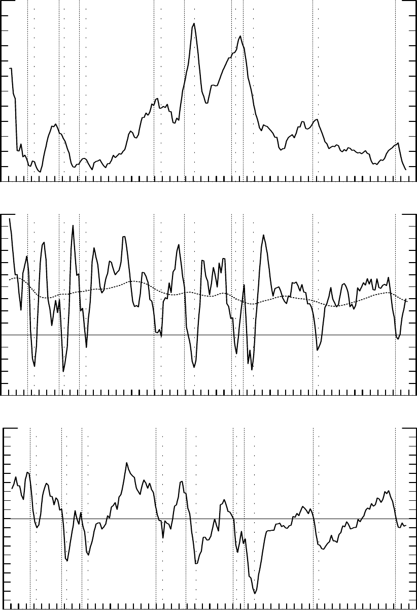
Figure 1. The U.S. Economy since the Accord
Inflation (Output Deflator)
0
1
2
3
4
5
6
7
8
9
10
11
12
1951 1955 1959 1963 1967 1971 1975 1979 1983 1987 1991 1995 1999 2003
Percent
Real Output Growth: Actual and Potential
-5
-4
-3
-2
-1
0
1
2
3
4
5
6
7
8
9
10
1951 1955 1959 1963 1967 1971 1975 1979 1983 1987 1991 1995 1999 2003
Percent
Output Gap
-10
-9
-8
-7
-6
-5
-4
-3
-2
-1
0
1
2
3
4
5
6
7
8
9
10
1951 1955 1959 1963 1967 1971 1975 1979 1983 1987 1991 1995 1999 2003
Percent
Notes: Inflation and growth are over four quarters. Dotted vertical lines denote NBER
peaks and troughs.
43

Figure 2. The Classic Taylor Rule
0
1
2
3
4
5
6
7
8
9
10
11
12
1982 1984 1986 1988 1990 1992 1994 1996 1998 2000 2002
Percent
Federal Funds
1992
2002
Real-Time
Notes: The 1992 rendition of the Taylor rule replicates the rule shown in Taylor (1993). The
solid vertical lines show the beginning and end of the sample originally discussed in Taylor
(1993). The 2002 rendition employs the latest data (Figure 1). The real-time rendition
employs, in every quarter, data as available in that quarter (Figure 3).
44

Figure 3. Real-Time and Retrospective Views of the Economy
Inflation
0
1
2
3
4
5
6
7
8
9
10
11
12
13
14
1951 1955 1959 1963 1967 1971 1975 1979 1983 1987 1991 1995 1999 2003
Percent
Inflation: 2002
Inflation: Real-Time
Real Output Growth: Actual and Potential
-7
-6
-5
-4
-3
-2
-1
0
1
2
3
4
5
6
7
8
9
10
11
12
1951 1955 1959 1963 1967 1971 1975 1979 1983 1987 1991 1995 1999 2003
Percent
2002
Real Time
Output Gap
-17
-16
-15
-14
-13
-12
-11
-10
-9
-8
-7
-6
-5
-4
-3
-2
-1
0
1
2
3
4
5
6
7
8
1951 1955 1959 1963 1967 1971 1975 1979 1983 1987 1991 1995 1999 2003
Percent
2002
Real-Time
Notes: One-quarter lagged values are plotted. Real-time data as discussed in the text. See
also notes to Figure 1.
45

Figure 4. Real-Time and Retrospective Classic Taylor Rule
-2
-1
0
1
2
3
4
5
6
7
8
9
10
11
12
13
14
15
16
17
18
19
20
1951 1955 1959 1963 1967 1971 1975 1979 1983 1987 1991 1995 1999 2003
Percent
Federal funds
Rule in 2002
Rule in Real Time
Notes: Real-time and retrospective renditions of the classic Taylor rule based on real-time
and retrospective data shown in Figure 3. Dotted vertical lines denote NBER peaks and
troughs.
46

Figure 5
Output Gap: Actual and Implied b y Classic Rule
-18
-16
-14
-12
-10
-8
-6
-4
-2
0
2
4
6
8
10
1961 1964 1967 1970 1973 1976 1979 1982 1985 1988 1991 1994 1997 2000
Percent
2002
Real Time
Implied by Taylor Rule
Evolution of Historical Output Gap Perceptions
-10
-9
-8
-7
-6
-5
-4
-3
-2
-1
0
1
2
3
4
5
6
7
8
1960 1962 1964 1966 1968 1970 1972 1974 1976 1978 1980 1982
Percent
1973
1982
1994
47

Figure 6
Forecast-Based Variants of the Classic R ule
0
1
2
3
4
5
6
7
8
9
10
11
12
13
14
15
16
17
18
19
20
1969 1972 1975 1978 1981 1984 1987 1990 1993 1996 1999 2002
Percent
Inflation Forecast/Output Gap Outcome
Inflation and Output Gap Forecast
Federal funds
Classic and Forecast-Based Natural-Growth Rule
0
1
2
3
4
5
6
7
8
9
10
11
12
13
14
15
16
17
18
19
20
1969 1972 1975 1978 1981 1984 1987 1990 1993 1996 1999 2002
Percent
Federal funds
Natural Growth Rule
Classic Rule
Notes: Forecasts are from the Greenbook until 1997Q4 and from the Survey of Professional
Forecasters from 1998Q1 on. The solid vertical line indicates the break in the data source.
Dotted vertical lines denote NBER peaks and troughs.
48

Figure 7. The High-Tide Years as a Prelude to the Crash
Price Indexes
80
90
100
110
120
130
140
150
160
170
1919 1920 1921 1922 1923 1924 1925 1926 1927 1928 1929
1926=100
Wholesale Commodities Prices
General Price Index
Industrial Production and Output Gap
60
70
80
90
100
110
120
130
1919 1920 1921 1922 1923 1924 1925 1926 1927 1928 1929
Industrial Production (1923-25=100)
Detrended Index of Industrial Production and Trade (Normal=100)
Interest Rates
2
3
4
5
6
7
8
1919 1920 1921 1922 1923 1924 1925 1926 1927 1928 1929
Percent
Discount
T-bill
49
