Learning R Markdown and Notebooks in RStudio

May 16, 2018

Contents

Introduction 3

Install LaTeX distribution via tinytex 4

Create a new R Notebook 4

The parts of an R Markdown document . . . . . . . . . . . . . . . . . . . . . . . . . . . . . . . . . . . . . . . . . . 4

YAML header . . . . . . . . . . . . . . . . . . . . . . . . . . . . . . . . . . . . . . . . . . . . . . . . . . . . . . 4

Text . . . . . . . . . . . . . . . . . . . . . . . . . . . . . . . . . . . . . . . . . . . . . . . . . . . . . . . . . . . 5

Chunks . . . . . . . . . . . . . . . . . . . . . . . . . . . . . . . . . . . . . . . . . . . . . . . . . . . . . . . . . 5

Previewing an R Notebook 5

Saving the R Notebook document . . . . . . . . . . . . . . . . . . . . . . . . . . . . . . . . . . . . . . . . . . . . . 5

The output document of an R Notebook . . . . . . . . . . . . . . . . . . . . . . . . . . . . . . . . . . . . . . . . . . 6

Code output appears only after running code . . . . . . . . . . . . . . . . . . . . . . . . . . . . . . . . . . . . . . . 6

Formatting plain text using Markdown 7

Headers . . . . . . . . . . . . . . . . . . . . . . . . . . . . . . . . . . . . . . . . . . . . . . . . . . . . . . . . . . . . 8

Emphasis with italics or bold text . . . . . . . . . . . . . . . . . . . . . . . . . . . . . . . . . . . . . . . . . . . . . 8

Bulleted and numbered lists . . . . . . . . . . . . . . . . . . . . . . . . . . . . . . . . . . . . . . . . . . . . . . . . . 8

Bulleted lists . . . . . . . . . . . . . . . . . . . . . . . . . . . . . . . . . . . . . . . . . . . . . . . . . . . . . . 8

Numbered lists . . . . . . . . . . . . . . . . . . . . . . . . . . . . . . . . . . . . . . . . . . . . . . . . . . . . . 8

Blockquotes . . . . . . . . . . . . . . . . . . . . . . . . . . . . . . . . . . . . . . . . . . . . . . . . . . . . . . . . . . 9

Links . . . . . . . . . . . . . . . . . . . . . . . . . . . . . . . . . . . . . . . . . . . . . . . . . . . . . . . . . . . . . . 9

Images . . . . . . . . . . . . . . . . . . . . . . . . . . . . . . . . . . . . . . . . . . . . . . . . . . . . . . . . . . . . . 10

Inline R code . . . . . . . . . . . . . . . . . . . . . . . . . . . . . . . . . . . . . . . . . . . . . . . . . . . . . . . . . 10

Plain code blocks . . . . . . . . . . . . . . . . . . . . . . . . . . . . . . . . . . . . . . . . . . . . . . . . . . . . . . . 11

Including equations in text . . . . . . . . . . . . . . . . . . . . . . . . . . . . . . . . . . . . . . . . . . . . . . . . . 11

Inline equations . . . . . . . . . . . . . . . . . . . . . . . . . . . . . . . . . . . . . . . . . . . . . . . . . . . . . 11

Display equation . . . . . . . . . . . . . . . . . . . . . . . . . . . . . . . . . . . . . . . . . . . . . . . . . . . . 11

Line breaks . . . . . . . . . . . . . . . . . . . . . . . . . . . . . . . . . . . . . . . . . . . . . . . . . . . . . . . . . . 11

Miscellaneous . . . . . . . . . . . . . . . . . . . . . . . . . . . . . . . . . . . . . . . . . . . . . . . . . . . . . . . . . 11

Superscripts . . . . . . . . . . . . . . . . . . . . . . . . . . . . . . . . . . . . . . . . . . . . . . . . . . . . . . . 12

Subscripts . . . . . . . . . . . . . . . . . . . . . . . . . . . . . . . . . . . . . . . . . . . . . . . . . . . . . . . . 12

Strikethroughs . . . . . . . . . . . . . . . . . . . . . . . . . . . . . . . . . . . . . . . . . . . . . . . . . . . . . 12

Going beyond Markdown basics . . . . . . . . . . . . . . . . . . . . . . . . . . . . . . . . . . . . . . . . . . . . . . . 12

YAML header 12

Adding title/date/author information to the document . . . . . . . . . . . . . . . . . . . . . . . . . . . . . . . . . . 12

Changing the format of the document . . . . . . . . . . . . . . . . . . . . . . . . . . . . . . . . . . . . . . . . . . . 13

Adding a table of contents . . . . . . . . . . . . . . . . . . . . . . . . . . . . . . . . . . . . . . . . . . . . . . . 13

Controlling the depth of the table of contents . . . . . . . . . . . . . . . . . . . . . . . . . . . . . . . . . . . . 13

A ﬂoating table of contents . . . . . . . . . . . . . . . . . . . . . . . . . . . . . . . . . . . . . . . . . . . . . . 14

Remove ﬁgure captions . . . . . . . . . . . . . . . . . . . . . . . . . . . . . . . . . . . . . . . . . . . . . . . . . 14

Figure height and width in the YAML header doesn’t work for R Notebooks . . . . . . . . . . . . . . . . . . . 14

Code chunks 15

Options to control chunk output . . . . . . . . . . . . . . . . . . . . . . . . . . . . . . . . . . . . . . . . . . . . . . 15

Suppressing messages and warnings: the message and warning options . . . . . . . . . . . . . . . . . . . . . . 15

Suppressing code output: the eval option . . . . . . . . . . . . . . . . . . . . . . . . . . . . . . . . . . . . . . 16

Suppressing code: the echo option . . . . . . . . . . . . . . . . . . . . . . . . . . . . . . . . . . . . . . . . . . 17

Controlling ﬁgure size . . . . . . . . . . . . . . . . . . . . . . . . . . . . . . . . . . . . . . . . . . . . . . . . . 18

The setup chunk . . . . . . . . . . . . . . . . . . . . . . . . . . . . . . . . . . . . . . . . . . . . . . . . . . . . . . . 21

Making a setup chunk . . . . . . . . . . . . . . . . . . . . . . . . . . . . . . . . . . . . . . . . . . . . . . . . . 21

Running all chunks again after adding a setup chunk . . . . . . . . . . . . . . . . . . . . . . . . . . . . . . . . 21

Default working directory for R Markdown documents 21

Reading a dataset based on the default working directory . . . . . . . . . . . . . . . . . . . . . . . . . . . . . . . . 21

Changing to a diﬀerent default directory . . . . . . . . . . . . . . . . . . . . . . . . . . . . . . . . . . . . . . . . . . 22

Other R Notebook features 22

Restarting an R Notebook after closing your R session . . . . . . . . . . . . . . . . . . . . . . . . . . . . . . . . . . 22

Separating single code chunks into multiples . . . . . . . . . . . . . . . . . . . . . . . . . . . . . . . . . . . . . . . . 22

Embedding interactive graphics . . . . . . . . . . . . . . . . . . . . . . . . . . . . . . . . . . . . . . . . . . . . . . . 23

Re-running all chunks . . . . . . . . . . . . . . . . . . . . . . . . . . . . . . . . . . . . . . . . . . . . . . . . . . . . 24

Create a PDF Markdown document 24

YAML header . . . . . . . . . . . . . . . . . . . . . . . . . . . . . . . . . . . . . . . . . . . . . . . . . . . . . . . . . 25

Setup chunk . . . . . . . . . . . . . . . . . . . . . . . . . . . . . . . . . . . . . . . . . . . . . . . . . . . . . . . . . . 25

R Markdown with PDF output 26

Saving the R Markdown document . . . . . . . . . . . . . . . . . . . . . . . . . . . . . . . . . . . . . . . . . . . . . 26

Knitting to PDF requires LaTeX . . . . . . . . . . . . . . . . . . . . . . . . . . . . . . . . . . . . . . . . . . . . . . 26

The output PDF document . . . . . . . . . . . . . . . . . . . . . . . . . . . . . . . . . . . . . . . . . . . . . . . . . 26

Code chunks always create output by default . . . . . . . . . . . . . . . . . . . . . . . . . . . . . . . . . . . . 26

Removing pound signs from code output via setup chunk . . . . . . . . . . . . . . . . . . . . . . . . . . . . . 27

YAML header options for PDF documents 27

Add table of contents . . . . . . . . . . . . . . . . . . . . . . . . . . . . . . . . . . . . . . . . . . . . . . . . . . . . 27

Change the document margins . . . . . . . . . . . . . . . . . . . . . . . . . . . . . . . . . . . . . . . . . . . . . . . 27

Make URL links visible . . . . . . . . . . . . . . . . . . . . . . . . . . . . . . . . . . . . . . . . . . . . . . . . . . . 28

More chunk options 28

A situation to use eval and echo . . . . . . . . . . . . . . . . . . . . . . . . . . . . . . . . . . . . . . . . . . . . . . 28

Holding ﬁgures to end of chunk with fig.show . . . . . . . . . . . . . . . . . . . . . . . . . . . . . . . . . . . . . . 29

Naming chunks . . . . . . . . . . . . . . . . . . . . . . . . . . . . . . . . . . . . . . . . . . . . . . . . . . . . . . . . 29

Chunk names in the navigation bar . . . . . . . . . . . . . . . . . . . . . . . . . . . . . . . . . . . . . . . . . . 30

Chunks with the same name . . . . . . . . . . . . . . . . . . . . . . . . . . . . . . . . . . . . . . . . . . . . . . 30

Knitting errors 30

Knitting an R Notebook to a PDF 31

Change how static images are added . . . . . . . . . . . . . . . . . . . . . . . . . . . . . . . . . . . . . . . . . . . . 31

Making interactive plots static while knitting . . . . . . . . . . . . . . . . . . . . . . . . . . . . . . . . . . . . . . . 31

Use always_allow_html in the YAML header . . . . . . . . . . . . . . . . . . . . . . . . . . . . . . . . . . . . 32

Use package webshot . . . . . . . . . . . . . . . . . . . . . . . . . . . . . . . . . . . . . . . . . . . . . . . . . 32

Make URL links visible . . . . . . . . . . . . . . . . . . . . . . . . . . . . . . . . . . . . . . . . . . . . . . . . . . . 32

Navigating with the outline side-bar 33

Options and links 33

Informational links . . . . . . . . . . . . . . . . . . . . . . . . . . . . . . . . . . . . . . . . . . . . . . . . . . . . . . 33

Package tinytex . . . . . . . . . . . . . . . . . . . . . . . . . . . . . . . . . . . . . . . . . . . . . . . . . . . . 33

RStudio cheatsheet . . . . . . . . . . . . . . . . . . . . . . . . . . . . . . . . . . . . . . . . . . . . . . . . . . . 33

Markdown basics . . . . . . . . . . . . . . . . . . . . . . . . . . . . . . . . . . . . . . . . . . . . . . . . . . . . 33

LaTeX mathematical symbols . . . . . . . . . . . . . . . . . . . . . . . . . . . . . . . . . . . . . . . . . . . . . 33

Formatting HTML documents . . . . . . . . . . . . . . . . . . . . . . . . . . . . . . . . . . . . . . . . . . . . . 33

Formatting PDF documents . . . . . . . . . . . . . . . . . . . . . . . . . . . . . . . . . . . . . . . . . . . . . . 34

knitr chunk options . . . . . . . . . . . . . . . . . . . . . . . . . . . . . . . . . . . . . . . . . . . . . . . . . . 34

An argument for relative ﬁle paths . . . . . . . . . . . . . . . . . . . . . . . . . . . . . . . . . . . . . . . . . . 34

Chunk caching . . . . . . . . . . . . . . . . . . . . . . . . . . . . . . . . . . . . . . . . . . . . . . . . . . . . . 34

Adding citations . . . . . . . . . . . . . . . . . . . . . . . . . . . . . . . . . . . . . . . . . . . . . . . . . . . . 34

Introduction

Today we are going to be talking about creating R Markdown Notebooks and other R Markdown documents via RStudio.

The work we are doing today can be done outside RStudio via R packages rmarkdown and knitr along with the Pandoc

software package. RStudio has bundled these in a way that makes creating these documents very easy.

R Markdown documents allow the integration of plain text, code, and output. This makes writing reports, sharing repro-

ducible analysis code with collaborators (including one of your main collaborators, future you), or simply including narrative

to explain the steps in our analysis straightforward. R Markdown Notebooks are a speciﬁc type of R Markdown document

that allows for literate programming, where you are directly interacting with R while producing a high-quality, reproducible

HTML document as output.

In this workshop we will be coding interactively. This is because inherent in what we are doing today is not only writing the

code, but seeing what the output looks like. I think that doing this work on the ﬂy together rather than having the code

already written will help understand that.

Install LaTeX distribution via tinytex

Later today we will be making PDF output documents, which means we need a LaTeX distribution. We can install one (even

without administrative privileges) using package tinytex. Read about this package here.

We start by installing package tinytex in R. This can be done by going to Packages pane in RStudio, clicking on the Install

button and typing in the name of the package. Alternatively we could run install.packages("tinytex") in the Console.

Once the package is installed we can use it to install the TinyTeX distribution via the install_tinytex() function. This

will take a few minutes and we’ll have to click OK to three messages and ignore the error message at the end if we are on a

Windows machine.

tinytex::install_tinytex()

When this is done, we’ll close RStudio before reopening and checking if things worked using is_tinytex and hoping to see

TRUE. We do.

tinytex:::is_tinytex()

[1] TRUE

Last, we add a package to TinyTeX that we’ll be using later today to save from having to do it later.

tinytex::tlmgr_install("ulem")

Create a new R Notebook

We will be talking about R Markdown documents in general as well as R Notebooks speciﬁcally. They are related; a Notebook

is a special case of R Markdown that acts in a particular way. We will start with R Notebooks, as I think these encompass

a niche that may be particularly useful for graduate students and others who are relatively new to R and analyses.

To easily create a new Notebook in RStudio, go to

File > New File > R Notebook

You will get an Untitled document. RStudio has some example text and code already in the document along with some basic

information to get you started.

The parts of an R Markdown document

In this new ﬁle you’ve opened, you can see the three basic parts of a R Markdown document. We will talk about each of

these brieﬂy now and then go through each section in greater detail.

YAML header

At the top, surrounded by sets of three dashes (---), is the YAML header. The YAML header is used to deﬁne the structure

of the document. We will be covering the syntax needed for YAML.

The default YAML header for an R Notebook looks like:

---

title: "R Notebook"

output: html_notebook

---

Text

Next in the document you see sentences of text. This text is written in plain text, and formatting can be controlled the R

version of Markdown syntax. We are able to do this via the rmarkdown package, which RStudio usually installs and uses

automatically (here in lab we may need to install it).

Chunks

The last part of an R Markdown document is what’s called a chunk. The chunk is where the R (or other language) code is

inserted into the document. A chunk always begins with three backticks (```) followed by curly braces where we deﬁne the

language the code chunk will be in. The chunk ends with another set of three backticks. The backtick on many keyboards

is found on the same key as the tilde.

The basic code chunk in the initial Untitled R Notebook document looks like this:

```{r}

plot(cars)

```

We will talk more extensively about YAML headers, writing text via the R Markdown language, and code chunks in a few

minutes.

Previewing an R Notebook

As mentioned in the introduction, R Notebooks were created as a method of literate programming. They allow the integration

of plain text, code, and output so you can, e.g, view your analysis code and output while keeping track of your thought process.

Unlike other R Markdown documents, R Notebooks are interactive. This means you run code and add output interactively

within the document as you work rather than writing the whole document and R code and then compiling the document

with output as a ﬁnal step. This makes R Notebooks more like keeping a scientiﬁc notebook and less like writing a report or

tutorial, although Notebooks can certainly be used for these latter tasks, as well.

In R Notebooks, we preview the document to create the output HTML document. Let’s see what that looks like by clicking

the Preview button at the top of Untitled R Notebook.

Saving the R Notebook document

As soon as you click the Preview button you will be asked to save the document. R Markdown documents must be saved

before you can view any output from them. Save this document as notebook_test.Rmd into a directory you have access to.

This is the same folder you should have saved the PNG ﬁle and dataset I sent you, with the dataset inside a folder called

Data.

We save our R Markdown ﬁle as an Rmd document, which is the ﬁle type for an R Markdown document.

Note that I have purposely not set my working directory. This will allow me to show you additional default features of R

Notebooks later in the workshop.

Once we save the document the output document is created and opens in a new window. If it doesn’t open, click the Preview

button again to see the output document. This document is in the same directory and has the same name as our Rmd ﬁle

but is an nb.html ﬁle. This is the ending given to these HTML R Notebooks.

By default the output document opens in a new window instead of the RStudio Viewer pane. You can change this to open

in the Viewer pane via

Tools > Global Options. . . > R Markdown

and choosing Viewer Pane from the Show output preview in: drop down menu.

On small monitor computers, opening in a new window may work better than trying to see how things look in the Viewer

pane.

The output document of an R Notebook

Let’s take a closer look at the output document, which is a speciﬁc type of HTML document ending in nb.html, shown

below.

We see an overall title, which was made in the YAML header of our Rmd document. The text shows up in paragraph form,

with diﬀerent types of text (like italic text) and hyperlinks seamlessly included. The R code included in the chunk is now in

a gray box, separated from the rest of the text.

In R Notebooks, we have some additional features. We have a Code drop-down menu, giving us the options.

Show All Code

Hide All Code

Download Rmd

By default all code we’ve chosen to include in the document is shown. Choosing Hide All Code hides all code for the entire

document. We won’t talk about the Download Rmd option today, but this allows a collaborator to extract the Rmd ﬁle from

the HTML document.

There is also a Hide button in the .nb.html document. This will be available for each chunk, allowing code to be hidden

one chunk at a time. After hiding, this button turns into a Code button, allowing us to show the code chunk once again.

Code output appears only after running code

In our initial output document, we see the code but no code output. In R Notebooks, you have to run the code chunk within

the Rmd document before it will be included in the output. This interactivity is a big diﬀerence between Notebooks and other

R Markdown documents.

Our initial document actually tells us how to run the code chunk: we either click the Run button within the chunk or put

the cursor inside the chunk and press Ctrl+Shift+Enter (OS X: Cmd+Shift+Enter). Let’s do that now.

The code output immediately shows up below the code chunk in our Rmd document. This is now the default in RStudio for

all Markdown documents (go to Global Options. . . to change this), but it is an inherent part of the nature of R Notebooks

coming into play; we write code and run it and have the output show up in our document interactively. Once we have run

the chunk we either save the Rmd or preview it to see it in the output document.

Formatting plain text using Markdown

Now that we have seen the basics, I want to talk about each part of an R Markdown document in more detail. I’m going

to start with showing how to control the plain text format via Markdown. Markdown is a simple formatting syntax. It has

relatively few options, which can be both good and bad.

I often can’t remember all of the syntax and have to go back and check how something works. The RStudio cheatsheet is a

good resource, as is RStudio’s Markdown Basics page.

Let’s practice Markdown by adding some plain text to notebook_doc.Rmd.

Headers

Headers in Markdown are indicated using the pound sign, #. We make headers of diﬀerent sizes using diﬀerent number of #.

These headers allow us to make a table of contents, so they are nice to include in an R Markdown document.

Add a header to indicate an Introduction to Markdown section. This will be a top-level header, so will have a single #.

# Introduction to Markdown

Our secondary header could be titled ## Headers, with some text about headers beneath it. You will see these changes in

the nb.html document when you save or push Preview again.

The text size of headers is set in the built-in documents in RStudio. In HTML documents they are large, as HTML documents

are meant for reading on the computer You’ll see headers in other formats, such as PDF documents, are generally smaller.

You can change header size of HTML documents, but you’d have to do it via CSS as shown in this Stack Overﬂow answer,

which we won’t cover today.

Emphasis with italics or bold text

We can use italics by wrapping text in single asterisks (*): *italic*.

Bold text is achieved with double asterisks (**): **bold**.

The initial text of our R Notebook has examples of italics. Add in a sentence with some bold text in it to see what it looks

like in the output document.

Bulleted and numbered lists

Bulleted lists

Making bulleted lists involves using a single asterisk (*), a plus signs (+), or a dash (-) at the start of each line, followed by a

space and then the list item. If you don’t have the space between the symbol and list item you won’t get bullets. We indent

with ≥ 4 spaces to get nested bullets.

Let’s try it in our practice Notebook.

* First bullet

* Second bullet

+ Secondary bullet

The output will look like:

• First bullet

• Second bullet

– Secondary bullet

Numbered lists

Making a numbered list is similar. We simply use numbers followed by a period and a space before each list item We can use

+ or * or letters/numbers to add bullets in a nested list. We’ll use letters today for the nested list. Again, we have to indent

with ≥ 4 spaces for the nested elements of the list to work properly.

1. Item 1

2. Item 2

3. Item 3

a. Item 3a

b. Item 3b

1. Item 1

2. Item 2

3. Item 3

a. Item 3a

b. Item 3b

You will notice that we need to make a new paragraph for this formatting to work. If we don’t, the text is viewed as plain

text that is part of the previous paragraph.

Try only using a single line break at the end of the previous paragraph or sentence instead of two and see how you get plain

text instead of a list.

Blockquotes

We use the greater than symbol, >, for blockquotes. As long as you don’t include two line breaks or spaces at the end of a

line, the text will wrap into a single blockquote.

> Here is how to write a block quote

as a single block of text even if it is written

on multiple lines

Here is how to write a block quote on a single line even if it is written on multiple lines

To do multiple block quotes in a row (vs a paragraph in a blockquote), end each line with two or more spaces. If you don’t

put the spaces at the end, the lines will run together on a single line.

> Here is the first block quote

> Here is the second

Here is the ﬁrst block quote

Here is the second

You can also put line breaks between the lines, but there will then be a line break between each blockquote.

> Here is the first block quote

> Here is the second

Here is the ﬁrst block quote

Here is the second

Links

Clickable links can be included by writing a URL in the text.

http://rmarkdown.rstudio.com

Alternatively, use brackets and parentheses to hide the address and allow the user to click on a word or phrase. This option

was included in the built-in text of our Notebook. The term R Markdown is the clickable link.

[R Markdown](http://rmarkdown.rstudio.com)

R Markdown

Images

We can add images in Markdown. We’ll need a path to the image, so we’ll either have the image saved to a folder we have

access to or have a web address where the image is stored (for HTML output only).

Including images involves brackets and parentheses much like including links, but the brackets are preceded by a exclamation

point (!).

In a presentation that’s powered by RStudio, we could include their logo by downloading an image of the logo from their

website. Let’s save the image at https://www.rstudio.com/wp-content/uploads/2014/07/RStudio-Logo-Blue-Gradient.png

into the folder we’re working in. While we can read it from the URL when making an HTML document, it won’t work if we

switch to a PDF document output so saving the image locally is the “safest” method.

![Caption](RStudio-Logo-Blue-Gradient.png)

We will get a caption by default. The caption is what you write within the square brackets. We can remove the caption by

making changes to the YAML header, which we’ll see soon. I have removed captions from this document, so the RStudio

logo I included below has no caption.

Jump to the [Images in a PDF document] section below for an alternative for inserting images that works well for all output

document types.

Inline R code

R code can be evaluated inline using single backticks, `, around a lower case r along with code. The r indicates the language

used in the code.

This can be useful if we want to pull something from some results we’ve made in R and put it within our text. Being able

to code it like this means we don’t have to copy/paste it in.

Here’s an example of what we would write in plain text, using backticks around a lowercase r followed by the R code to

evaluate.

There were `r nrow(mtcars)` rows in the dataset.

And this is what the result would look like in the output document.

There were 32 rows in the dataset.

Generally, inline R code should be relatively simple as it will be evaluated every time the document is saved. Code that takes

a long time to run should likely be put in a code chunk.

Plain code blocks

If we are trying to include an example of syntax that we don’t want evaluated, we can wrap it in triple backticks much like

a code chunk. Unlike code chunks, plain code blocks have no curly braces that indicate the language of the code.

Here’s what code would look like if we were showing someone how to use asterisks for italic text.

```

Write in *italics* with single asterisks.

```

Below is what it would look like in the output document.

Write in *italics* with single asterisks.

Including equations in text

Equations or Greek letters can be included within text using LaTeX equations wrapped in dollar signs. We will not go into

details on LaTeX equations, but see here for a list of LaTeX mathematical symbols.

Inline equations

You can include equations within a sentence using single dollar signs. Symbols are preceded by a backslash, \.

Let's talk about $\sigma^2$ within a sentence, using the Greek letter.

Let’s talk about σ

within a sentence, using the Greek letter.

Display equation

To display an equation on its own line, use double dollar signs.

Here is how we sum everything together: $$\sum_{i=1}^n X_i$$

Here is how we sum everything together:

i=1

Line breaks

Force new pages by putting three or more dashes or asterisks on a line.

****

----

Miscellaneous

You can use superscripts, subscripts, and strikethroughs in Markdown syntax, as well.

Superscripts

Superscripts can be indicated with carets, ˆ, around the symbol we want in superscript.

y^2^

Subscripts

Subscripts can be indicated with single tildes, ~, around the subscripted symbol.

H~2~O

Strikethroughs

Strikethroughs are indicated with double tildes, ~~, around the terms we want to strike out.

~~Strike this out~~

Strike this out

Going beyond Markdown basics

Markdown syntax, as you can see, is pretty simple. This means you are limited in how much formatting you can do in

Markdown. If you want or need to do more complicated things in your Markdown document than what is listed above,

you are able to do so. However, that usually will mean writing some code in an alternative syntax such as CSS or LaTeX

(depending on the format of the output document). When I am in this situation, I end up searching online and can usually

ﬁnd what I’m looking for and add it to the document.

YAML header

We will next talk about things we can add or change in the YAML header to change the structure of the document.

By default, RStudio ﬁlls in the output type based on the kind of document we chose to open. Because we are working with

an R Notebook, you can see that the output is an html_notebook. RStudio also includes an overall title in the YAML

header, which we may or may not want.

There are many things we can add or change in the YAML header. Many of these options are outlined at the RStudio HTML

R Markdown page. The link above is speciﬁc to HTML documents; for PDF documents see the PDF R Markdown page.

Controlling the appearance of the diﬀerent output document types can take diﬀerent commands.

Adding title/date/author information to the document

Some of the basic things we can add to the document are titles, authors, and dates. We could also remove the title all

together by deleting that line.

The title is included by default by RStudio. Let’s change it to “Practice Notebook”. Let’s add the date while we’re at it.

The date option is date:. Each option in the YAML header has a colon after it followed by a space.

---

title: "Practice Notebook"

date: May 16, 2018

output: html_notebook

---

We can add author information, as well.

---

title: "Practice Notebook"

date: May 16, 2018

author: Ariel Muldoon

output: html_notebook

---

Changing the format of the document

Many of the changes we make to the document are done as options to html_notebook.

If we look at the help page for html_notebook, which we can do via ?html_notebook, we see some of the options we can

control in our output document.

html_notebook(toc = FALSE, toc_depth = 3, toc_float = FALSE,

number_sections = FALSE, fig_width = 7, fig_height = 5,

fig_retina = 2, fig_caption = TRUE, code_folding = "show",

smart = TRUE, theme = "default", highlight = "textmate",

mathjax = "default", extra_dependencies = NULL, css = NULL,

includes = NULL, md_extensions = NULL, pandoc_args = NULL,

output_source = NULL, self_contained = TRUE, ...)

You can see there are many things you can control, from deciding whether you want to produce typographically correct output

automatically using smart (which defaults to TRUE) to controlling whether or not you get ﬁgure captions via fig_caption

(which also defaults to TRUE) and beyond.

We’ll hit on only a few of these so you can see what the code looks like. After each change we make, we’ll save or preview

the document to see how things have changed.

Adding a table of contents

We can add a table of contents using the toc option. As you can see on the help page, it defaults to FALSE. To get an

automatic table of contents based on the headers we’ve made we change this to TRUE.

We use a new format for the YAML header once we are changing options away from the defaults. This format is important;

things won’t work how you want if you don’t use the correct formatting.

To get the correct formatting, we add a line break after output: and indent two spaces before html_document:. We add

the colon after html_document. We then do another line break and indent another two spaces for including html_document

options that we can see from the help page listed above. In this case we will add toc: TRUE.

Below is what that will look like. Again, the formatting is important. If you don’t indent before an option within

html_document it will not take eﬀect.

---

title: "Practice Notebook"

date: May 16, 2018

author: Ariel Muldoon

output:

html_notebook:

toc: TRUE

---

Controlling the depth of the table of contents

The default table of contents depth for R Notebooks is 3. This means that the ﬁrst 3 levels of headers will be included in the

table of contents; i.e., headers created using #, ##, and ###. That may be too many or too few depending on the audience

of the output document. Let’s change the depth to 2.

When using multiple options within html_notebook, we continue with new line breaks but don’t indent any further. All the

arguments that are speciﬁc to html_notebook will then line up in our YAML header in a single column.

---

title: "Practice Notebook"

date: May 16, 2018

author: Ariel Muldoon

output:

html_notebook:

toc: TRUE

toc_depth: 2

---

A ﬂoating table of contents

In HTML R Markdown documents such as Notebooks, we can allow the table of contents to “ﬂoat”. This means it will move

when we scroll through the document. This is controlled via toc_float, which by default is FALSE.

You cannot have a ﬂoating table of contents in a static document such as a PDF document. If you go to the help page for

pdf_document, you will see that toc_float is not an option.

---

title: "Practice Notebook"

date: May 16, 2018

author: Ariel Muldoon

output:

html_notebook:

toc: TRUE

toc_depth: 2

toc_float: TRUE

---

There are additional options to control what the ﬂoating table of contents looks like. By default it is collapsed, which isn’t

always ideal. See the link I gave above for an example of adding sub-options to the html_document options.

Remove ﬁgure captions

We can get rid of captions on images via the fig_caption: FALSE option of the YAML header. Let’s do that now. Upon

previewing, we will see the caption is gone on our RStudio logo image.

---

title: "Practice Notebook"

date: May 16, 2018

author: Ariel Muldoon

output:

html_notebook:

toc: TRUE

toc_depth: 2

toc_float: TRUE

fig_caption: FALSE

---

Figure height and width in the YAML header doesn’t work for R Notebooks

You see in the help document for html_notebook that there are options for controlling fig_width and fig_height. However,

those do not currently work with R Notebooks. We will instead control ﬁgure height and width via chunk options.

Code chunks

Now that we’ve gotten the text and formatting bits out of the way, let’s get down to business and talk about the code chunks.

We will be writing code chunks in R, although you can write and include output from code chunks from other languages such

as Python and Stan in R Markdown documents.

We’ll start by including a code chunk to load packages. I often have a chunk like this at the beginning of a document. We’ll

load some packages I know we have installed in this room. If you’re on your own computer, you may need to install these.

As our initial document tells us, we can insert a new chunk using Ctrl+Alt+I (Mac OS Cmd+Option+I ). We can also simply

type out the ``` and {r} ourselves.

The code chunk will look like this:

```{r}

library(ggplot2)

library(dplyr)

```

Let’s run the chunk. We see the green line, indicating R is running through the lines of code.

In this case, we also see the output, which is a warning about the R version and then several messages we get from dplyr.

library(ggplot2)

library(dplyr)

Attaching package: 'dplyr'

The following objects are masked from 'package:stats':

filter, lag

The following objects are masked from 'package:base':

intersect, setdiff, setequal, union

Options to control chunk output

These package messages can be important, but there are times when we might not want them in our ﬁnal document. We

can control what and how chunks print using the options provided by the knitr package. This package is what’s working

under the hood to put the R output in our output document.

There are, perhaps unsurprisingly, a ton of chunk options. The author of the knitr package, Yihui Xie, goes through the

chunk options on his website, https://yihui.name/knitr/options/. I often end up reading through these when I’m trying to

ﬁgure out how to get the output I want.

Suppressing messages and warnings: the message and warning options

We can keep messages from printing with the message option. This option is logical, and defaults to TRUE, meaning messages

are printed in the chunk output. Below is the description of message.

message: (TRUE; logical) whether to preserve messages emitted by message() (similar to warning)

If we want to remove messages we need to set message to FALSE in the chunk header. The chunk header is everything that

is within the curly braces at the beginning of the chunk.

If we get output like package dplyr was built under R version 3.3.3, that’s a warning, not a message. We control

warnings with the warning option. This is also logical and also defaults to TRUE. See also the error option.

warning: (TRUE; logical) whether to preserve warnings (produced by warning()) in the output like we run R

code in a terminal (if FALSE, all warnings will be printed in the console instead of the output document); it can

also take numeric values as indices to select a subset of warnings to include in the output

R Notebooks are interactive, meaning the code is run in real time. So before we can test if the output has changed when

we change the chunk header, we need to unload the packages via detach. Then we can load them again to see if the chunk

options worked.

detach("package:dplyr", unload = TRUE)

detach("package:ggplot2", unload = TRUE)

Now that the packages are detached, we will rerun the package chunk after adding message = FALSE in the chunk header.

We add these within the curly braces. It’s common to put a comma after r before writing the chunk options. This has to do

with naming chunks, which we will discuss later.

Here is what the new code chunk looks like.

```{r, message = FALSE}

library(dplyr)

library(ggplot2)

```

Now when we run this, we’ll see the green line showing code is running in our R Notebook but we will not get the message

in our output.

library(ggplot2)

library(dplyr)

Suppressing code output: the eval option

Sometimes we are going to write a chunk to show R code in our output, but we don’t actually want the code to run or the

output to be included in the ﬁnal document. We can use eval for this.

eval: (TRUE; logical) whether to evaluate the code chunk; it can also be a numeric vector to select which R

expression(s) to evaluate, e.g. eval=c(1, 3, 4) or eval=-(4:5)

This is less common to use in an R Notebook than other R Markdown documents, as usually we speciﬁcally want the output

to show in ﬁnal document. However, I use this a lot for teaching documents where I’m doing something like showing code to

go to a help page that I don’t actually want to run.

As an example, sometimes I want to put some tabular output into a nicer looking table rather than using the default R

output. So while I want my audience to see the R code used to make the tabular output, I use other tools to make the table

look more attractive in the document. In this case I need to suppress the code output from the code chunk.

We can see this by making a summary dataset with dplyr.

```{r}

mtcars %>%

group_by(cyl) %>%

summarise(mdisp = mean(disp) )

```

mtcars %>%

group_by(cyl) %>%

summarise(mdisp = mean(disp) )

# A tibble: 3 x 2

cyl mdisp

1 4.00 105

2 6.00 183

3 8.00 353

I can suppress the output to show the code output in a diﬀerent format. This can be one adding eval = FALSE to the chunk

header.

```{r, eval = FALSE}

mtcars %>%

group_by(cyl) %>%

summarise( mdisp = mean(disp) )

```

We run the code and it still shows up in our Rmd ﬁle. However, when we look at the preview we see the summary output

doesn’t show since the code wasn’t evaluated.

mtcars %>%

group_by(cyl) %>%

summarise( mdisp = mean(disp) )

We’ll expand on this example later in the workshop to show a simple way to make a nicer looking table as output.

Suppressing code: the echo option

I commonly ﬁnd I want to show output but not code when making R Markdown documents. This is what the echo option

is for. See the similar include option, as well.

echo: (TRUE; logical or numeric) whether to include R source code in the output ﬁle; besides TRUE/FALSE

which completely turns on/oﬀ the source code, we can also use a numeric vector to select which R expression(s)

to echo in a chunk, e.g. echo=2:3 means only echo the 2nd and 3rd expressions, and echo=-4 means to exclude

the 4th expression

A plot is something we’d commonly want in our output but, depending on our audience, we may not want to show the R

code that made the plot.

Let’s make a plot using the built-in dataset mtcars.

```{r}

qplot(wt, mpg, data = mtcars)

```

qplot(wt, mpg, data = mtcars)

2 3 4 5

mpg

If we wanted to show only the plot, without showing the code, we’ll use echo = FALSE in the chunk header.

```{r, echo = FALSE}

qplot(wt, mpg, data = mtcars)

```

2 3 4 5

mpg

Controlling ﬁgure size

R Notebooks have a speciﬁc ﬁgure height and width. While we can’t control ﬁgure size in R Notebooks via the YAML

header, we can control ﬁgure size via chunk options.

Let’s make the cars plot from the beginning of our practice notebook, but change the size of the ﬁgure. We do this via

fig.height and fig.width, setting the numeric size of the plot in inches.

```{r, fig.height = 10, fig.width = 5}

plot(cars)

```

The plot is now much taller and skinnier than our original plot.

plot(cars)

5 10 15 20 25

0 20 40 60 80 100 120

speed

dist

There are many more chunk options than we have time to talk about today. We’ll explore just a couple more, but we will

wait until we switch to working with an R Markdown document that is not a Notebook.

The setup chunk

Sometimes we may want to set the same chunk option for every chunk in the document, which can be tedious. We can

instead set options overall in the setup chunk using opts_chunk$set from knitr.

The setup chunk goes at the top of a Rmd document, right under the YAML header. We won’t want anyone to see that code

in the ﬁnal document, so we’ll use echo = FALSE in the setup chunk header.

It’s also nice to name the chunk so we (and R) will know it’s the setup chunk and can jump to it if we need. We can name

a chunk by typing a name (that contains no spaces) after the r in the chunk header. The name goes before the comma for

the chunk options.

Making a setup chunk

In our practice setup chunk we’ll set the plot size for all plots to be the same. We’ll add the setup chunk below to the top of

our practice Rmd ﬁle. As opts_chunk comes from package knitr, we load that package.

```{r setup, echo = FALSE}

library(knitr)

opts_chunk$set(fig.height = 10, fig.width = 5)

```

Running all chunks again after adding a setup chunk

Once we’ve created the setup chunk we’ll want to rerun all the chunks in our Rmd prior to previewing. This is because our R

Notebook is interactive, and the output we’ve already created in the document won’t change until we run the chunk again.

I’ve had a hard time remembering this behavior of R Notebooks, and have wondered why a chunk option was having no

eﬀect on the output. We must always rerun a chunk in an R Notebook to see any changes.

We can run all current chunks by choosing Run All Chunks under the Run button or by using the keyboard short-cut

Ctrl+Alt+R (OS X Command+Option+R).

Default working directory for R Markdown documents

The default working directory for R Notebooks and all other R Markdown documents is the directory where the Rmd ﬁle is

stored. This allows us to write all directory paths relative to that directory. This is helpful if we’ve organized things in such

a way that our Rmd ﬁle is in the root directory, i.e., the overall directory that your project data/scripts are stored in.

We can check this by adding and running a chunk to get the working directory, getwd, within our Rmd ﬁle. Remember, we

purposely did not set the working directory to the folder we are working in at the beginning of the workshop.

```{r}

getwd()

```

Run getwd() in the Console to see where the default working directory is for RStudio compared to the default working

directory of our R Notebook.

Reading a dataset based on the default working directory

Knowing that our Rmd ﬁle sets the default working directory to the directory it is located in allows us to organize our ﬁle

structure in such a way to take advantage of that default. I sent you a ﬁle called test.csv that I asked you to save in a

folder called Data in the folder you are working in today (the folder you are working in today is where you saved your Rmd

ﬁle). Let’s read that dataset in now.

When reading from a folder within our directory, we don’t have to write out the entire directory path. Instead, we can write

out the path starting at the folder within the default directory. You can see how that looks below. The . indicates the

directory path to the default directory, so we add on the folder and document name to that path.

dat = read.csv("./Data/test.csv")

dat

Diffmeans Lower.CI Upper.CI plantdate stocktype

1 -0.27 -0.63 0.09 Jan2 cont

2 0.11 -0.25 0.47 Jan28 cont

3 -0.15 -0.51 0.21 Jan28 bare

4 -1.27 -1.63 -0.91 Feb25 cont

5 -1.18 -1.54 -0.82 Feb25 bare

Changing to a diﬀerent default directory

There are package options that can be set via knitr that allows us to change the overall defaults, which we could do in the

setup chunk using opts_knit$set. This is a lot like how we set our chunk options. To change the default directory we can

use root.dir and deﬁne a new ﬁle path.

root.dir: (NULL) the root directory when evaluating code chunks; if NULL, the directory of the input document

will be used

The setwd function you may be used to using will not work in an R Markdown document. If you are working with a more

complicated directory structure but are taking advantage of RStudio Projects, using root.dir and here::here() together

can be useful for setting the root directory without hard-coding the default ﬁle path. Here is what the code you add to

the setup chunk could look like (using an actual ﬁle path where I wrote “ﬁlepath”): knitr::opts_knit$set(root.dir =

"filepath").

Working with relative paths instead of hard-coding paths is desirable. It allows for portability and reproducibility. If you

haven’t already, see the information about relative ﬁle paths here and check out the here package.

Other R Notebook features

We’re going to switch to working on another kind of R Markdown document, but we’ll ﬁrst cover a few more things that are

speciﬁc to R Notebooks.

Restarting an R Notebook after closing your R session

Remember that R Notebooks are interactive, as they are meant to mirror a scientiﬁc notebook. This means you run code

and see the code output within the document, and the ﬁnal document is based on the code you’ve actually run. If you go

back to a Notebook that you’ve already started after ending the session, you may need to run some or all of the chunks

before you can get do with any new R work that is based on previous work in the document. The Run button at the top of

the document has many options, and the buttons within each chunk have options, such as Run All Chunks Above, for this

reason.

Separating single code chunks into multiples

When working with R Notebooks, it is most common to place any code that creates R output into a single chunk rather than

having multiple outputs from a single chunk. This has to do with the scientiﬁc notebook/literate programming nature of

Notebooks, where you are describing what you are doing with the analysis/code/output in plain text. If you have two lines

of code in a single chunk, as shown below, you can easily separate them into two chunks by highlighting one of the lines of

code and then using Ctrl+Alt+I. This remove that line of code and puts it into a new chunk.

For example, I might have copied and pasted and code chunk into my document with two plots in it.

```{r}

qplot(disp, mpg, data = mtcars)

qplot(wt, mpg, data = mtcars)

```

If I want to separate this into separate chunks so I can easily comment on the two plots in text, I could highlight the second

line of code, qplot(wt, mpg, data = mtcars), and use the chunk keyboard shortcut or Insert button to get two chunks:

```{r}

qplot(disp, mpg, data = mtcars)

```

```{r}

qplot(wt, mpg, data = mtcars)

```

Embedding interactive graphics

Another thing we can do with R Notebooks is to insert interactive graphics into our Rmd and our output HTML using packages

such as dygraphs or plotly (note: plotly graphs don’t always work well in Firefox, but display ﬁne in, e.g., Chrome). Other

HTML-producing Markdown documents can also include interactive graphics in the output. Interactive graphics can be a

valuable tool for exploring the dataset and including them in an R Notebook allows us to share these with our collaborators

without, e.g., making and uploading a Shiny app.

Here is a plot, made using the dygraph function from the dygraphs package, that allows the limits of the x axis to change

interactively via a slider. The values of the x and y axis are shown in a tooltip when you hover over the plot. You may need

to install dygraphs prior to running this code if you’ve never used this package before.

Generally a plot made with dygraph will be a time series, although it can be numeric. See the documentation for more

information.

If you are reading the PDF version of this document, this plot will not be interactive but instead will be a small, static

graphic.

library(dygraphs)

dygraph(nhtemp) %>%

dyRangeSelector( dateWindow = c("1920-01-01", "1960-01-01") )

1920

1930

1940

1950

Re-running all chunks

When I make a Notebook for teaching purposes, I usually do a quick spell check using the ABC button, save everything, and

then use the Run option Restart R and Run All Chunks. I do this to ensure all my code works properly in a clean R session

in case I did something in R during my interactive work that I didn’t explicitly include in the Notebook. This works well for

relatively small documents, and is valuable when I’m making a document to send to someone else that needs to work exactly

as I have written it.

If you have a very large document that has R processes that take a long time to run, you likely won’t make use of this option

as often. One of the good thing about an R Notebook is that once you’ve run something and produced output you have it

in the document (both in the Rmd and the nb.html after saving). This makes it so you don’t need to run the chunk every

time you update the document.

Create a PDF Markdown document

Let’s close our Notebook and switch gears to working with another R Markdown document. This time we’ll make a document

that we will convert to a PDF.

To easily create a new Markdown document in RStudio, go to

File > New File > R Markdown. . .

You will get a pop-up window to ask what type of Markdown ﬁle you want to make (Document, Presentation, Shiny or From

Template) and what kind of default output format you want (HTML, PDF, or Word). You can also ﬁll in the title and

author for the YAML header.

We’ll choose to make a Markdown document with a PDF output. We will not be talking about the other ﬁle types today.

We’ll ﬁll in the title and author info today but we could delete them both to leave the YAML header blank.

Press OK and we get a new, untitled document in our Source Pane. It also has default text and code, so we’ll start by taking

a closer look at those.

YAML header

The included YAML header is very similar to our YAML header when we opened the new Notebook. Because we ﬁlled in a

title and author, those are ﬁlled in. We also get the date. Any of these can be removed as desired.

The primary diﬀerence is in the document type listed under output. Before we had a html_notebook; now we have a

pdf_document.

Our initial YAML header for a PDF Markdown document looks like:

---

title: "Workshop practice PDF"

author: "Ariel Muldoon"

date: "May 16, 2018"

output: pdf_document

---

Setup chunk

You can see the ﬁrst chunk is a setup chunk. This is included by default in new documents because it is so common to

have one. This particular setup chunk doesn’t do much, but it can easily be added to. Notice that it uses include = FALSE

instead of echo = FALSE to suppress the setup code from the output document

```{r setup, include=FALSE}

knitr::opts_chunk$set(echo = TRUE)

```

There are two other chunks in the default document. If we run them we do get output to show within the document by

default. However, running or not running chunks interactively will not aﬀect our output document. We won’t run these

chunks right now so we can see what happens in the output.

Note that you can stop output from showing within the Rmd document by going to

Global Options. . . > R Markdown

and unclick the box next to Show output inline for all R Markdown documents

R Markdown with PDF output

Instead of a Preview button at the top of the document, we now have a Knit button. This is what we will use to knit the

Rmd ﬁle to the output type we’ve chosen. In this case we’ll be knitting this document to a PDF, as we chose a PDF document

when we created the new R Markdown ﬁle.

This process is called knitting because the knitr package is doing the work behind the scenes.

Saving the R Markdown document

If you hit Knit, you will be prompted to save the document. Let’s save this as a document called pdf_test.Rmd.

Once you hit Save the document will immediately begin to knit. We can see the process in the R Markdown pane in RStudio,

which shows in the same pane as the Console. This is RStudio using various R packages and software to do the heavy lifting

of converting our Rmd to a PDF.

You’ll see RStudio keeps track of how much of the document has been knit. For small documents it seems almost instanta-

neous, but for larger documents this can help you keep track of the progress that has been made.

Knitting to PDF requires LaTeX

RStudio does this knitting in a way that looks pretty magical. However, we need a LaTeX program installed if we want

to knit a Markdown document to a non-HTML format, which is why we installed TinyTeX earlier. Other common LaTeX

distributions are MikTeX (Windows) and MacTeX (Mac OS).

If you do not have some version of LaTeX installed or RStudio can’t ﬁnd the one you do have, you will get errors when trying

to knit to non-HTML formats and you will need to troubleshoot.

The output PDF document

Once the PDF document has been created, we can take a closer look at it. You’ll see all the same elements as our R Notebook,

including information from the YAML header, plain text, and code with output.

Code chunks always create output by default

One thing I want you to see is that our two non-setup R code chunks both ran and the R output shows in the PDF document.

This is one big diﬀerence between interactive R Markdown Notebooks and non-interactive (or batch) R Markdown documents.

In the former, we run chunks interactively and they show up in the ﬁnal document. The document is updated each time you

save, but doesn’t run through any chunks that have already been run and saved previously.

In the latter, all code chunks are run every time you knit. The order the chunks are in is very important, as the chunks are

run in the order they show up in the document. This means you must have a code chunk that loads a package before a code

chunk that uses functions from that package.

For large R Markdown documents with a lot of slow code, running all chunks every time you knit can get tiresome. The

chunk option cache = TRUE can help with this, allowing the output to be cached after it is run the ﬁrst time to save on

processing time. See the caching page on the knitr author’s website for more info.

Removing pound signs from code output via setup chunk

If you look at the code output in the PDF, you’ll see each line is prefaced by two pound signs (##). My personal preference

is to remove those, and so I usually include comment = NA in the setup chunk to get rid of those.

We can change the setup chunk and re-knit to see the eﬀect.

```{r setup, include=FALSE}

knitr::opts_chunk$set(echo = TRUE, comment = NA)

```

YAML header options for PDF documents

As you already know, PDF documents have some distinct YAML header options. Review those here.

We can add YAML header options after pdf_document, much like we did in our Notebook earlier with html_notebook. See

the help page for pdf_document for more information and some of the options, shown below.

pdf_document(toc = FALSE, toc_depth = 2, number_sections = FALSE, ﬁg_width = 6.5, ﬁg_height = 4.5,

ﬁg_crop = TRUE, ﬁg_caption = TRUE, dev = “pdf”, df_print = “default”, highlight = “default”, template =

“default”, keep_tex = FALSE, latex_engine = “pdﬂatex”, citation_package = c(“none”, “natbib”, “biblatex”),

includes = NULL, md_extensions = NULL, pandoc_args = NULL, extra_dependencies = NULL)

You see that there is no option for a ﬂoating table of contents. We can’t have this kind of interactive element in static

documents like a PDF document, although the table of contents and links will still be clickable.

While we won’t cover it today, note there are options to add citations to a Markdown document; if you are interested see

here to get started. See also package bookdown.

Add table of contents

We won’t do much with more with the YAML header than we have already, but we will add a table of contents to the top

of the document based on the headers. Notice that we once again change the format of the header to add the indentations

and line breaks. Page numbers for each header are included in the table of contents.

---

title: "Workshop practice PDF"

author: "Ariel Muldoon"

date: "May 16, 2018"

output:

pdf_document:

toc: TRUE

---

Change the document margins

Other things I often change are things like the margins of the document. I ﬁnd this especially true when trying to get

ﬁgures to ﬁt nicely without leaving large blank spaces. Sometimes making the margins a little wider or narrower really helps.

Margins can be changed via geometry, setting the margins overall or just some of the margins. Here we’ll change all the

margins to 0.5 inches except the bottom margin, which will be set to 0.75 inches.

---

title: "Workshop practice PDF"

author: "Ariel Muldoon"

date: "May 16, 2018"

geometry: margin=.5in, bottom=.75in

output:

pdf_document:

toc: TRUE

---

Make URL links visible

In the HTML document, URL links were blue, so were easy to see. If you take a look at the PDF output document, you can

see the URL is clickable if you hover over it but otherwise it looks like the rest of the text. We can make these more visible

by changing the color using the urlcolor option in the YAML header. Today we’ll make URL links blue.

---

title: "Workshop practice PDF"

author: "Ariel Muldoon"

date: "May 16, 2018"

geometry: margin=.5in, bottom=.75in

urlcolor: blue

output:

pdf_document:

toc: TRUE

---

More chunk options

Let’s add a couple more code chunks so we can practice using chunk options.

A situation to use eval and echo

I outlined a situation earlier where I sometimes use eval. This is where I want to show the code for some tabular output, but

want the output to look nicer than it does by default. I can make the nicer output using a second chunk of code, suppressing

the code in that chunk from the output document using echo.

Let’s load dplyr here and remake that little summary table from earlier. All packages used within the R Markdown document

need to be loaded, regardless of if you’ve already loaded them interactively in your R session.

We still use Ctrl+Alt+I for inserting new code chunks in our new R Markdown document.

Below are what the three chunks could look like.

1. I load the package, using message = FALSE to suppress the loading messages.

2. I write the summary table code to include in the document, but suppress the output via eval = FALSE.

3. I make a nicer looking table in the output using the kable function from package knitr. I don’t want the code I use

for this to show in the document, so I use echo = FALSE.

The kable function is a relatively simple function with few options, but the output tables can be pretty nice looking without

much work in a PDF document.

```{r, message = FALSE}

library(dplyr)

```

```{r, eval = FALSE}

mtcars %>%

group_by(cyl) %>%

summarise(mdisp = mean(disp) )

```

```{r, echo = FALSE}

knitr::kable(mtcars %>%

group_by(cyl) %>%

summarise(mdisp = mean(disp) ) )

```

The code and output is below, although the eﬀect will not be the same if you are reading this in an nb.html document

compared to a PDF document.

library(dplyr)

mtcars %>%

group_by(cyl) %>%

summarise( mdisp = mean(disp) )

cyl mdisp

4 105.1364

6 183.3143

8 353.1000

Holding ﬁgures to end of chunk with fig.show

If making several plots in one code chunk, we can either allow each to show after the line of code has run or hold all of the

plots until the end of the chunk based on fig.show. By default, each plotted as soon as its line of code has been run.

ﬁg.show: (‘asis’; character) how to show/arrange the plots; four possible values are -asis: show plots exactly in

places where they were generated (as if the code were run in an R terminal); -hold: hold all plots and output

them in the very end of a code chunk; -animate: wrap all plots into an animation if there are mutiple plots in a

chunk; -hide: generate plot ﬁles but hide them in the output document

Let’s make two plots in one code chunk. After knitting we see what happens by default, which is that we see the plot shown

immediately after the line of code that produced it.

```{r}

plot(cars)

plot(pressure)

```

Using fig.show = "hold", we hold all plots to be produced at the end of the chunk. This does not work in R Notebooks so

I don’t show the output here.

```{r, fig.show = "hold"}

plot(cars)

plot(pressure)

```

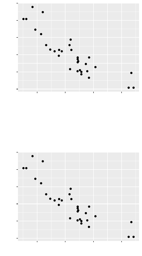
If we change the width of the ﬁgures, we can get them to ﬁt next to each other. This saves us some space.

```{r, fig.show = "hold", fig.width = 4}

plot(cars)

plot(pressure)

```

Naming chunks

We named the setup chunk earlier, but haven’t talked any more about naming chunks. I name chunks in most of my long

Markdown documents, as it improves my ability to jump around in the document.

Each chunk must have a unique name. If you make the mistake of repeating a chunk name you will get an error on knitting.

Let’s add a chunk name to our last code chunk. We’ll name it twoplots. We add this after the r but before the comma in

the chunk header.

```{r twoplots, fig.show = "hold", fig.width = 4}

plot(cars)

plot(pressure)

```

Chunk names in the navigation bar

When you click on the navigation bar in the lower left corner of the document, you can see all headers and chunks. The

chunks are numbered by default, and when we add names, the names are also be listed. This can make organization and

navigation within an R Markdown document easier.

Chunks with the same name

To see what happens when two chunks have the same name, change the last chunk name to pressure. There is already a

chunk named pressure in this document. Now attempt to knit the document.

We see an error in the R Markdown pane:

processing ﬁle: pdf_test.Rmd Error in parse_block(g[-1], g[1], params.src) : duplicate label ‘pressure’ Calls: . . .

process_ﬁle -> split_ﬁle -> lapply -> FUN -> parse_block Execution halted

Among all the other words, the error clearly tells us we have a duplicate label and what that label is, allowing us to go and

ﬁx it.

Knitting errors

What about other knitting errors? If we have R code that has an error in it and won’t run, the knitting will fail. The message

we get will look diﬃcult to read initially, but it does indicate a line number within the Rmd ﬁle as a starting point for ﬁnding

the error.

Change the last chunk name back to twoplots, and remove the closing parenthesis in one line of plot code. Failing to close

parentheses in R means code can’t ﬁnish running.

```{r twoplots, fig.show = "hold", fig.width = 4}

plot(cars)

plot(pressure

```

In the Output part of the R Markdown pane we’ll see an error message directly after R attempted to run the twoplots chunk.

This is where chunk names can once again be helpful. We also get the line numbers of the chunk that is causing issues.

Quitting from lines 55-57 (pdf_test.Rmd) Error in parse(text = x, srcﬁle = src) : :3:0: unexpected end of input 1:

plot(cars) 2: plot(pressure ˆ Calls: . . . evaluate -> parse_all -> parse_all.character -> parse Execution halted

In the Issues part of the pane we’ll see a line number and the same message written again. This line number is the ﬁrst line

of the chunk that is causing the issue. We can now navigate to that chunk and see if we can ﬁgure out what the problem is.

Knitting an R Notebook to a PDF

The last thing we’ll do is go back to our practice notebook ﬁle, notebook_test.Rmd, and knit it to a PDF. The HTML output

notebook has a lot of good things about it, including the way the Rmd ﬁle is embedded in it. However, HTML ﬁles tend not

to be very good for printing and sometimes we’ll want to take the ﬁle and make a PDF ﬁle in addition to the nb.html ﬁle.

We can knit to a PDF by going to the drop down menu arrow next to Preview and choosing Knit to PDF. However, we have

several elements in the R Notebook that work for HTML output that won’t work well for a static PDF output. Let’s make

a few changes before proceeding.

Change how static images are added

Inserting images via the Markdown language as we did earlier doesn’t always work well for PDF output documents. Images

aren’t necessarily placed exactly where you put them but instead the computer places them wherever it ﬁnds enough space.

A convenient alternative is to use R code to insert graphics using insert_graphics() from package knitr instead of using

Markdown syntax. The width of the output is controlled by the code chunk option out.width and the code can be suppressed

using echo = FALSE.

Here is what the code looks like to insert the RStudio logo via knitr, which will replace our R Markdown syntax. As this

also works for HTML output formats, this is likely the best default option for inserting images. Remember that for nb.html

output ﬁles we’ll need to run this code before the image will appear in the output.

```{r, echo = FALSE, out.width = "100%"}

knitr::include_graphics('RStudio-Logo-Blue-Gradient.png')

```

Using this option puts the image right where you want it, regardless of the output document type. I put mine below.

Making interactive plots static while knitting

Interactive graphics only work for HTML output ﬁles. If we try to knit to a PDF document with an interactive graphic we’ll

see an error message:

Error: Functions that produce HTML output found in document targeting latex output. Please change the output

type of this document to HTML. Alternatively, you can allow HTML output in non-HTML formats by adding

this option to the YAML front-matter of your rmarkdown ﬁle:

always_allow_html: yes

Note however that the HTML output will not be visible in non-HTML formats.

Execution halted

Use always_allow_html in the YAML header

One option to avoid problems of interactive graphs in static documents is to add always_allow_html: yes to our YAML

header. This suppresses the interactive graphic in the resulting static document, so it simply doesn’t print at all.

Adding that would look like:

---

title: "Practice Notebook"

date: May 16, 2018

author: Ariel Muldoon

always_allow_html: yes

output:

html_notebook:

toc: TRUE

toc_depth: 2

toc_float: TRUE

fig_caption: FALSE

---

Use package webshot

The nicer option is it install package webshot and the install PhantomJS with webshot::install_phantomjs(). This

allows knitr to take a static image of our interactive graphic and include it in the PDF. If we use this option we don’t need

to add anything to the YAML header.

Make URL links visible

If we have URL links in our document, we might want to use the urlcolor YAML header option to make URL links visible.

---

title: "Practice Notebook"

date: May 16, 2018

author: Ariel Muldoon

urlcolor: blue

output:

html_notebook:

toc: TRUE

toc_depth: 2

toc_float: TRUE

fig_caption: FALSE

---

Once we’ve made the changes outlined above, we can knit things to a PDF via the drop down menu. RStudio edits the

YAML header for us to indicate we are now knitting to a PDF document. You’ll see we have a second output type listed.

Once we Knit to PDF, the pdf_document output is listed ﬁrst and the YAML header looks like what’s printed below. RStudio

also changed some of our TRUE/FALSE to yes/no, but that doesn’t change the resulting document.

---

title: "Practice Notebook"

author: "Ariel Muldoon"

date: "May 16, 2018"

output:

pdf_document:

toc: yes

toc_depth: '2'

html_notebook:

fig_caption: no

toc: yes

toc_depth: 2

toc_float: yes

urlcolor: blue

---

We could make further changes to the YAML header that are speciﬁc to the PDF document output, as needed.

To go back to the HTML output, we switch the order of the output in the YAML header manually or choose Preview Notebook

from the drop down menu.

Navigating with the outline side-bar

In addition to the Navigation bar at the bottom that we saw when discussing code chunks, we can navigate through an R

Markdown document via the headers by opening the outline side-bar. The default is to not show the outline (although this

can be changed in Global Options. . . > R Markdown). I often use the outline to navigate, which can be opened by clicking

on the button in the upper right corner of the R Markdown document:

Options and links

I’ve given you a basic start to learn how to take advantage of R Notebooks and other R Markdown documents. While we

didn’t see it today, there is an option to knit Rmd ﬁles to Word documents.

These same tools can also be extended to making slides for presentations, allowing you to include R code and/or output

within the rest of your slides.

Informational links

Throughout this document outlining the workshop, I’ve given you links to pages that cover important material. I’ll end by

listing the complete address for each one here. There is a lot of information about these topics on the internet, and these are

a good starting point if you get stuck.

Package tinytex

https://yihui.name/tinytex/

RStudio cheatsheet

https://www.rstudio.com/wp-content/uploads/2015/02/rmarkdown-cheatsheet.pdf

Markdown basics

http://rmarkdown.rstudio.com/authoring_basics.html

LaTeX mathematical symbols

https://oeis.org/wiki/List_of_LaTeX_mathematical_symbols

Formatting HTML documents

http://rmarkdown.rstudio.com/html_document_format.html#overview

Formatting PDF documents

http://rmarkdown.rstudio.com/pdf_document_format.html#overview

knitr chunk options

https://yihui.name/knitr/options/

An argument for relative ﬁle paths

https://www.tidyverse.org/articles/2017/12/workﬂow-vs-script/

Chunk caching

https://yihui.name/knitr/demo/cache/

Adding citations

http://rmarkdown.rstudio.com/authoring_bibliographies_and_citations.html