
University of Arkansas, Fayetteville University of Arkansas, Fayetteville
ScholarWorks@UARK ScholarWorks@UARK
Chemical Engineering Undergraduate Honors
Theses
Chemical Engineering
5-2023
Heat Transfer from Plates Heat Transfer from Plates
Leanza Trevino
Follow this and additional works at: https://scholarworks.uark.edu/cheguht
Part of the Thermodynamics Commons, and the Transport Phenomena Commons
Citation Citation
Trevino, L. (2023). Heat Transfer from Plates.
Chemical Engineering Undergraduate Honors Theses
Retrieved from https://scholarworks.uark.edu/cheguht/191
This Thesis is brought to you for free and open access by the Chemical Engineering at ScholarWorks@UARK. It has
been accepted for inclusion in Chemical Engineering Undergraduate Honors Theses by an authorized administrator
of ScholarWorks@UARK. For more information, please contact [email protected].
Heat Transfer from Plates
Leanza Treviño
A Thesis Presented to Committee on Undergraduate Studies
in the
College of Engineering, Ralph E. Martin Department of Chemical Engineering
in Partial Fulfillment of the Requirements
for the Degree with Honors
of Bachelor of Science in Chemical Engineering
University of Arkansas
Fayetteville, Arkansas
March 2023
Contents
I. Summary
II. Introduction
III. Experimental Approach
IV. Calculations Approach
V. Results
VI. Discussion
VII. Appendix
a. Free Convection Heat Transfer from Plates Handout
b. Forced Convection Heat Transfer from Plates Handout
List of Figures
1. Experimental Apparatus
2. Run 1. Free Convection 4 Oct 2022
3. Run 1. Forced Convection 11 Oct 2022, 130 V
4. Run 2. Free Convection 4 Oct 2022
5. Run 3. Free Convection 4 Oct 2022
6. Run 2. Forced Convection 11 Oct 2022, 130 V
7. Run 3. Forced Convection 31 Oct 2022, 90 V
8. Run 4. Forced Convection 31 Oct 2022, 90 V
List of Tables
1. Free Convection Experimental Data Summary
2. Forced Convection Experimental Data Summary
3. Summary of Relevant Data for Run 1. Free Convection
4. Summary of Relevant Data for Run 1. Forced Convection
Summary
The purpose of this honors thesis is to create an experiment for the CHEG Lab I course. This is a
continuation of work done by Alexa Moreno. She created an experiment to model free
convection of a horizontal plate. In this report, free and forced convection of a vertical and
horizontal plate, respectively are modeled. This report explains the motivation for creating this
heat convection experiment, the results of performing the experiment, and provides
recommendations for future work on this experiment.
Introduction
Undergraduate students pursuing a chemical engineering degree must successfully complete the
chemical engineering Lab I and Lab II courses. The purpose of this honors thesis is to create an
experiment for the Lab I course.
Previous work performed by Alexa Moreno modeled free convection of a horizontal plate. Over
the course of nine experiments, she produced data with an average error of 13.05% as compared
to a theoretical model. The same equipment was used for the experiments discussed here, with
some additions for the forced convection experiment.
Students will be tasked to study free convective heat transfer by monitoring temperature changes
over time for an aluminum plate that has been heated and allowed to cool in an insulated stand
with the vertical face being exposed to atmospheric temperature and pressure. Forced convective
heat transfer is studied by monitoring temperature changes over time for an aluminum plate that
has been heated and allowed to cool in an insulated stand with the vertical face being exposed to
forced convection via a set of fans blowing over the surface. The students will record
experimental data and determine a best fit experimental heat transfer coefficient by using
MATLAB to solve a differential equation for the heat balance. In addition, a theoretical heat
transfer coefficient will be determined from empirical correlations (Cengel 2007, Table 9-1, p.
511). The experimental and theoretical heat transfer coefficients will be compared and discussed.
Recommendations for further improvement include a more rigorous calculations approach that
does not assume constant film properties.
Experimental Approach
The aluminum plate was painted black on the face that is to be exposed to air because the
emissivity coefficient of black paint is known. The emissivity coefficient is used in the
calculations for the experimental heat transfer coefficient. An insulated stand was built to prevent
heat loss on all other sides of the plate aside from the face painted black. The stand was
constructed with PVC material and built with enough room to have thermal insulation
underneath the plate and around the sides of the plate. A hole was drilled in the stand, insulation,
and plate large enough for a thermocouple wire to fit to monitor temperature changes over time.
An oven, already owned by the chemical engineering department, was used to heat the aluminum
plate as displayed in Figure 1.

Figure 1. Experimental Apparatus
A 0.5” plate was used for the experiment. The desired temperature range to monitor was 75°C to
45°C. Multiple runs were executed to ensure that the data extracted would prove beneficial for
students to replicate and discuss. The total time for the experiment takes 50-60 minutes for one
plate to heat and cool long enough to see the entire temperature range desired.
As Lab I is allotted a longer time slot, students may perform back-to-back experiments modeling
both free and forced or free horizontal and vertical convection with the use of a second
aluminum plate. This requires placing the second plate in the oven upon removal of the first.
Running the series of two takes approximately 90 minutes.

Calculations Approach
Once sufficient data was collected, MATLAB’s ode45 function was used to model the
experiment. To determine the experimental heat transfer coefficient, the heat transfer coefficient
was manually changed to determine the value at which the integrated differential equation best
matched the experimental data plotted. This is a brute force method and most certainly not the
most efficient way to find the coefficient. However, Lab I students have limited coding
experience, so this method is a good approach for a beginner to try. In the future, more advanced,
iteration-loop-based coding along with defining a metric to determine how well two lines match
each other could be applied to find the exact number for the experimental heat transfer
coefficient.
Results
A summary of the experiment time and errors for three free convection runs is displayed
below in Table 1. Table 2 is a similar summary for forced convection results.
Table 1. Free Convection Experimental Data Summary
Run
Total Run Time (min)
Percent Error
1
53
17.1
2
60
23.3
3
46
17.1
Average
53
19.2
Table 2. Forced Convection Experimental Data Summary
Run
Total Run Time (min)
Percent Error
1
41
47.7
2
36
45.9
3
39
50.9
4*
50
49.9
Average
41.5
48.6
*Run 4 was left in oven too long, time to reach desired high temperature was approximately 10
minutes less than actual time left heating in oven.
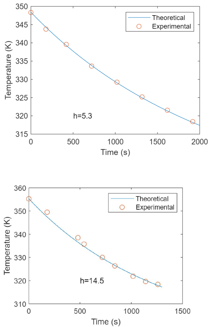
Figures 2 and 3 show the experimental data from free and forced convection runs with low
percentage errors.
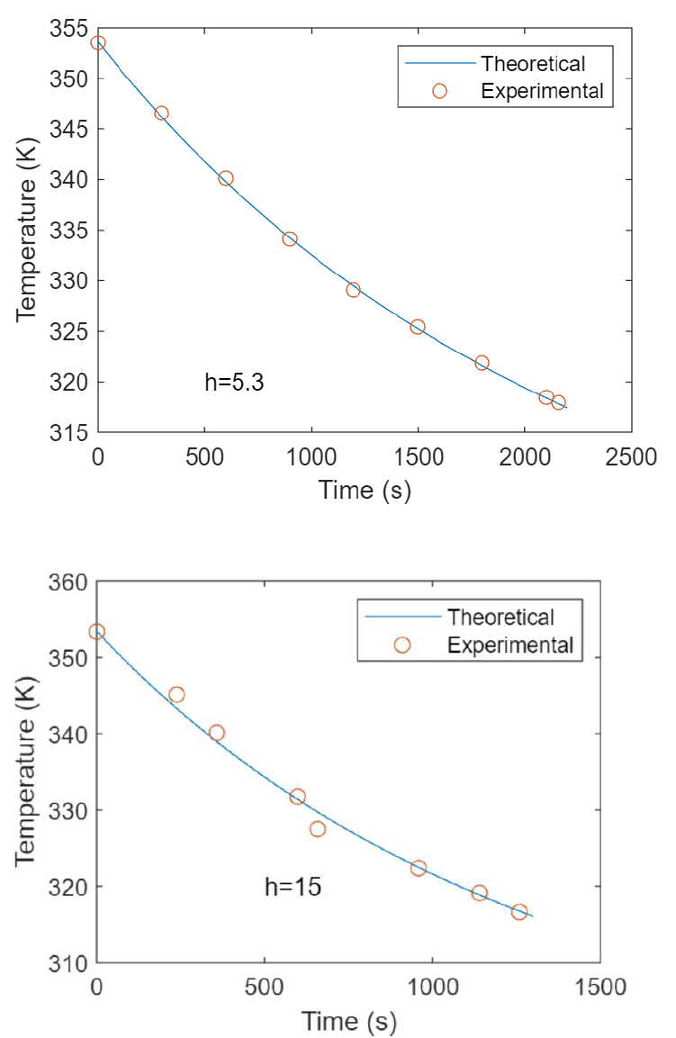
Figure 2. Run 1. Free Convection 4 Oct 2022
Figure 3. Run 1. Forced Convection 11 Oct 2022, 130 V
A summary of relevant data for these runs are displayed in Tables 3 and 4. These are used to
determine the percent error and integrity of the experiment.

Table 3. Summary of Relevant Data for Run 1 Free
Value
Units
h
CORR
6.39
h
EXP
5.3
Tplate
80.6
°C
Table 4. Summary of Relevant Data for Run 1 Forced
Value
Units
h
CORR
7.85
h
EXP
15
Tplate
80.4
°C
V at 130V
2.54
m/s
Discussion
As previously determined in work by Alexa Moreno, MATLAB is an effective tool for analyzing
the data. The experimental heat transfer coefficient for free convection was consistently less than
the calculated theoretical heat transfer coefficient.
The experimental heat transfer coefficient for forced convection was consistently greater than
theoretical. The significantly larger percent difference in this data could be a result of incorrect
windspeeds. The stand made for the vertical experiment causes inconsistent wind flow across the
surface. For the experimental value, the measurement was taken at the point above the
thermocouple. However, minor differences in the location resulted in notable windspeed
variances. The overall discrepancies for forced and free convection can also be accounted for by
noting the use of constant parameter assumptions. This is not true for the actual situation as the
film temperature is changing throughout, thus altering various other values.
Conclusion
Both a forced and free convection experiment can be performed in a Lab I session. Handouts for
both cases were created and are available in the Appendix. Experimental and theoretical data
correlated closely for free convection experiments. In forced convection experiments the
experimental heat transfer coefficient was consistently higher than the theoretically calculated
value, but this provides further discussion points for future students. For future improvement of
the forced convection calculations, the changing film temperature could be accounted for.

Appendix
Data Reduction
A heat balance on the center plate, with no heat generation, yields Equation 1:
ACCOUT
qq =−
(1)
The plate is cooled by free convection and radiation, as is shown in Equation 2:
(2)
The plate accumulates heat with an inverse relationship to time as it cools back to room-
temperature, noted in Equation 3:
( ) ( )
dt
dT
CV
dt
dT
Cmq
ppACC
==
(3)
Thus, the heat balance of Equation 1 yields Equation 4:
(4)
Experimental temperature data will be used to determine the “best fit” experimental heat
transfer coefficient by integrating Equation 4 using MATLAB’s ode45 function.
The heat transfer coefficient from the literature can be determined using the correlation for
free convection from a horizontal heated, horizontal-facing plate
(Cengel 2007, p. 511, Table
9-1), shown in Equations 5.
(5)
where the Rayleigh number is calculated as in Equation 6:
(6)
The heat transfer coefficient from the literature can be determined using the correlation for
forced convection from a heated, horizontal-facing plate
(Cengel 2007, p. 402), shown in
Equations 5a and 5b:
(7a)
(7b)
where the Reynolds number is calculated as in Equation 7 (constants from Cengel 2007,
Equation 6-13, p.366):
(8)

In Equation 6, the depth of the plate is the characteristic length in free convection for a
horizontal flat plate. Finally, h
CORR
may be calculated from the Nusselt number as shown in
Equation 7:
L
kNu
h
CORR
=
(9)
The experimental coefficient will be higher than the coefficient calculated from a literature
correlation since it is impossible to remove all forced convection influences and achieve only
free convection.
Sample Calculation
Free Convection
The theoretical heat transfer coefficient, h
CORR
, is calculated using the equation below:
Nu is calculated by finding the Rayleigh number, where
, with T being the internal
temperature of the plate at 356.4 K, g equal to 9.81 m/s
2
, equal to 0.00002085 m
2
/s, and
Prandtl number of air equal to 0.7157.
Because the Rayleigh number is in magnitude of
, equation 5a is used to calculate Nu.
The fluid thermal conductivity of air, k, is 0.02945 W/mK. Therefore,
The experimental heat transfer coefficient, h
EXP
, was found to be 6.35. The percent error can be
calculated using the following equation:
Applying this formula, the percent error for this experimental run would be:

Forced Convection
The theoretical heat transfer coefficient, h
CORR
, is calculated using the equation below:
Nu is calculated by finding the Reynolds number where the density and viscosity of air at room
temperature are used. The characteristic length of the plate is 0.6096 m, and the velocity is 2.54
m/s.
Because the Reynolds number is less than the magnitude of
, equation 5a is used to calculate
Nu. The Prandtl number of air is 0.7157.
The fluid thermal conductivity of air, k, is 0.02945 W/mK. Therefore,
The experimental heat transfer coefficient, h
EXP
, was found to be 6.35. The percent error can be
calculated using the following equation:
Applying this formula, the percent error for this experimental run would be:

Sample Code
Free Convection
The following code was used to find the theoretical values for the run shown in the sample
calculation along with a figure. This code produces Figure 1 shown earlier.

Forced Convection
The following code was used to find the theoretical values for the run shown in the sample
calculation along with a figure. This code produces Figure 1 shown earlier.

Figures
Run 2. Free Convection 4 Oct 2022
Run 3. Free Convection 4 Oct 2022
Run 2. Forced Convection 11 Oct 2022, 130 V

Run 3. Forced Convection 31 Oct 2022, 90 V
Run 4. Forced Convection 31 Oct 2022, 90 V

Ralph E. Martin Department of Chemical Engineering
University of Arkansas
Fayetteville, AR
CHEG 4332L
CHEMICAL ENGINEERING LABORATORY II
FREE CONVECTION HEAT TRANSFER FROM PLATES
Authors: Edgar C. Clausen (University of Arkansas), W. Roy Penney (University of Arkansas),
Alexa Moreno (University of Arkansas), Leanza Trevino (University of Arkansas)
PURPOSE
The purpose of this experiment is to provide the students with experience modeling free
convection heat transfer from an aluminum plate in the vertical position. Also, the students will
apply heat transfer theory by determining experimental and theoretical heat transfer coefficients.
The students will become familiar with MATLAB’s ode45 function and scatter plot capabilities.
REPORT
1. Plot the experimental data using MATLAB’s scatter plot function.
2. Generate model plot using MATLAB’s ode45 function.
3. Using the model plot, determine the experimental free convection heat transfer
coefficient for the surface of a vertical hot plate exposed to air.
4. Compare the results with results generated from the appropriate correlation of Churchill
and Chu
(Cengal 2007).
REFERENCES
1. Cengel, Y.A. 2007. Heat and Mass Transfer: A Practical Approach, Chapter 9: Natural
Convection. Pages 503-560. 3
rd
edition. Boston: McGraw-Hill.
2. Omega Engineering. 2017. Emissivity of Common Materials. No date. Accessed August
14, 2017. https://www.omega.com/literature/transactions/volume1/emissivitya.html.

PROCEDURE
Equipment Description
The aluminum plate (24”x13”x0.5”, 6.51 kg) is heated to 85°C inside the Fisher Oven. To keep
record of the plate temperature, a thermocouple is inserted in the center of the plate with the oven
door closed, as shown in Figure 1. To ensure that heat does not escape the oven, a rubber stopper
is used to seal the hole at the top of the oven, as shown in Figure 2. A thermocouple is also used
to monitor the temperature of the inside of the oven, also pictured in Figure 2.
Figure 1. Experimental Apparatus inside Fisher Oven.

Figure 2. Rubber Stopper.
After the desired internal temperature is reached, the plate is moved to a 27.5” x 15.5” x 3” PVC
stand, black side showing, surrounded by thermal insulation on the back of the plate and the
sides of the plate. The thermocouple is inserted in the side of the stand through the drilled in hole
in line with the drilled hole in the aluminum plate to monitor the temperature changes over time
as shown in Figure 3.
Figure 3. Experimental Apparatus for Cooling
Materials and Equipment Needed
The following equipment are used in carrying out this experiment:
• Oven
• Aluminum Plate, painted black on one face with a hold drilled from one side to the center
• Insulation (THERMAX Sheathing, 3.3 R factor per ½” of board)
• PVC Stand
• Stopwatch
• Thermocouple Reader
• Two Thermocouple Wires
• Rubber Stopper
• Pry Bar
Procedure
1. Safety precautions that must be followed during the experiment include:
a. Wear proper PPE, including safety goggles, long sleeve shirt, long pants, closed
toed shoes.
b. Wear fire-safe lab coat, thermal arm sleeves, and high heat-resistant gloves when
opening the oven and transferring the heated plate.
c. Use pry bar when lifting the aluminum plate out of insulation and transferring to
oven.
d. Be sure to have group members steer clear of path when transferring the
aluminum plate.
2. The oven will be pre-heated by the TA. Ensure all PPE is worn before opening the oven
door. Lift the aluminum plate with the pry bar and transfer to the inside of the oven as
seen in Figure 1.
3. Insert the shorter thermocouple wire into the hole at the top of the oven, avoiding
touching the plate, to monitor the temperature inside the oven (make sure the oven is
never losing temperature). Hold the wire in place with rubber stopper, shown in Figure 2.
4. Slide the longer thermocouple wire through the hole in the side of the aluminum plate
and shut the oven door.
5. Wait for the aluminum plate to reach an internal temperature of 85°C.
6. Once the desired temperature is reached, remove the rubber stopper and remove the
thermocouple wire from inside the oven.
7. Be sure all PPE is worn, open the oven door, pull thermocouple wire out of the hole,
transfer plate to insulated stand and insulate the last side of the aluminum plate.
8. Insert the longer thermocouple wire into the side of the insulation stand to the center of
the plate, as shown in Figure 3.
9. Start the stopwatch as soon as the temperature is no longer climbing and record the initial
temperature.
10. Record the temperature every 3 minutes until the temperature reaches 45°C.
11. Stop the stopwatch. Remove the thermocouple wire from the side of the plate. Shut off
the thermocouple reader and clean the area, putting away all PPE.

APPENDIX
1. Data Reduction
A heat balance on the center plate, with no heat generation, yields Equation 1:
ACCOUT
qq =−
(1)
The plate is cooled by free convection and radiation, as is shown in Equation 2:
(2)
The plate accumulates heat with an inverse relationship to time as it cools back to room-
temperature, noted in Equation 3:
( ) ( )
dt
dT
CV
dt
dT
Cmq
ppACC
==
(3)
Thus, the heat balance of Equation 1 yields Equation 4:
(4)
Experimental temperature data will be used to determine the “best fit” experimental heat
transfer coefficient by integrating Equation 4 using MATLAB’s ode45 function.
The heat transfer coefficient from the literature can be determined using the correlation for
free convection from a heated, vertical-facing plate
(Cengal 2007, p. 402), shown in
Equations 5.
(5)
where the Rayleigh number is calculated as in Equation 6:
(6)
In Equation 6, the depth of the plate is the characteristic length in free convection for a
horizontal flat plate. Finally, h
CORR
may be calculated from the Nusselt number as shown in
Equation 8:
L
kNu
h
CORR
=
(8)
The experimental coefficient will be higher than the coefficient calculated from a literature
correlation since it is impossible to remove all forced convection influences and achieve only
free convection.

Ralph E. Martin Department of Chemical Engineering
University of Arkansas
Fayetteville, AR
CHEG 4332L
CHEMICAL ENGINEERING LABORATORY II
FORCED CONVECTION HEAT TRANSFER FROM PLATES
Authors: Edgar C. Clausen (University of Arkansas), W. Roy Penney (University of Arkansas),
Alexa Moreno (University of Arkansas), Leanza Trevino (University of Arkansas)
PURPOSE
The purpose of this experiment is to provide the students with experience modeling forced
convection heat transfer from an aluminum plate in the vertical position. Also, the students will
apply heat transfer theory by determining experimental and theoretical heat transfer coefficients.
The students will become familiar with MATLAB’s ode45 function and scatter plot capabilities.
REPORT
1. Plot the experimental data using MATLAB’s scatter plot function.
2. Generate model plot using MATLAB’s ode45 function.
3. Using the model plot, determine the experimental forced convection heat transfer
coefficient for the top surface of a vertical hot plate with forced convection.
4. Compare the results with results generated from the appropriate correlation of
Churchill and Chu
(Cengal 2007).
REFERENCES
1. Cengel, Y.A. 2007. Heat and Mass Transfer: A Practical Approach, Chapter 9: Natural
Convection. Pages 503-560. 3
rd
edition. Boston: McGraw-Hill.
2. Omega Engineering. 2017. Emissivity of Common Materials. No date. Accessed August
14, 2017. https://www.omega.com/literature/transactions/volume1/emissivitya.html.

PROCEDURE
Equipment Description
The aluminum plate (24”x13”x0.5”, 6.51 kg) is heated to 85°C inside the Fisher Oven. To keep
record of the plate temperature, a thermocouple is inserted in the center of the plate with the oven
door closed, as shown in Figure 1. To ensure that heat does not escape the oven, a rubber stopper
is used to seal the hole at the top of the oven, as shown in Figure 2. A thermocouple is also used
to monitor the temperature of the inside of the oven, also pictured in Figure 2.
Figure 1. Experimental Apparatus inside Fisher Oven.

Figure 2. Rubber Stopper.
After the desired internal temperature is reached, the plate is moved to a 27.5” x 15.5” x 3” PVC
stand, black side showing, surrounded by thermal insulation on the back of the plate and the
sides of the plate. The thermocouple is inserted in the side of the stand through the drilled in hole
in line with the drilled hole in the aluminum plate to monitor the temperature changes over time.
A series of fans are aimed at the plate as shown in Figure 3.
Figure 3. Equipment Setup.
Materials and Equipment Needed
The following equipment are used in carrying out this experiment:
• Oven
• Aluminum Plate, painted black on one face with a hold drilled from one side to the center
• Insulation (THERMAX Sheathing, 3.3 R factor per ½” of board)
• PVC Stand
• Stopwatch
• Thermocouple Reader
• Two Thermocouple Wires
• Rubber Stopper
• Pry Bar
Procedure
12. Safety precautions that must be followed during the experiment include:
a. Wear proper PPE, including safety goggles, long sleeve shirt, long pants, closed
toed shoes.
b. Wear fire-safe lab coat, thermal arm sleeves, and high heat-resistant gloves when
opening the oven and transferring the heated plate.
c. Use pry bar when lifting the aluminum plate out of insulation and transferring to
oven.
d. Be sure to have group members steer clear of path when transferring the
aluminum plate.
13. The oven will be pre-heated by the TA. Ensure all PPE is worn before opening the oven
door. Lift the aluminum plate with the pry bar and transfer to the inside of the oven as
seen in Figure 1.
14. Insert the shorter thermocouple wire into the hole at the top of the oven, avoiding
touching the plate, to monitor the temperature inside the oven (make sure the oven is
never losing temperature). Hold the wire in place with rubber stopper, shown in Figure 2.
15. Slide the longer thermocouple wire through the hole in the side of the aluminum plate
and shut the oven door.
16. Wait for the aluminum plate to reach an internal temperature of 85°C.
17. Once the desired temperature is reached, remove the rubber stopper and remove the
thermocouple wire from inside the oven.
18. Be sure all PPE is worn, open the oven door, pull thermocouple wire out of the hole,
transfer plate to insulated stand and insulate the last side of the aluminum plate.
19. Insert the longer thermocouple wire into the side of the insulation stand to the center of
the plate, as shown in Figure 3.
20. Turn on the fans and record windspeed at the point above the thermocouple’s internal
position in the plate.
21. Start the stopwatch as soon as the temperature is no longer climbing and record the initial
temperature.
22. Record the temperature every 3 minutes until the temperature reaches 45°C.
23. Stop the stopwatch. Remove the thermocouple wire from the side of the plate. Shut off
the thermocouple reader and clean the area, putting away all PPE.

APPENDIX
3. Data Reduction
A heat balance on the center plate, with no heat generation, yields Equation 1:
ACCOUT
qq =−
(1)
The plate is cooled by free convection and radiation, as is shown in Equation 2:
(2)
The plate accumulates heat with an inverse relationship to time as it cools back to room-
temperature, noted in Equation 3:
( ) ( )
dt
dT
CV
dt
dT
Cmq
ppACC
==
(3)
Thus, the heat balance of Equation 1 yields Equation 4:
(4)
Experimental temperature data will be used to determine the “best fit” experimental heat
transfer coefficient by integrating Equation 4 using MATLAB’s ode45 function.
The heat transfer coefficient from the literature can be determined using the correlation for
free convection from a horizontal heated, horizontal-facing plate
(Cengal 2007, p. 402),
shown in Equations 5a and 5b:
(5a)
(5b)
where the Reynolds number is calculated as in Equation 6 (constants from Cengal 2007,
Equation 6-13, p.366):
(6)
In Equation 6, the depth of the plate is the characteristic length in free convection for a
horizontal flat plate. Finally, h
CORR
may be calculated from the Nusselt number as shown in
Equation 7:
L
kNu
h
CORR
=
(7)
The experimental coefficient will be higher than the coefficient calculated from a literature
correlation since it is impossible to remove all forced convection influences and achieve only
free convection.

4. Nomenclature
A
S
area for convection, m
2
C
p
specific heat of the aluminum plate or cylinder, J/kg K
g gravitational constant, m/s
2
h convection heat transfer coefficient, W/m
2
K
h
CORR
correlated heat transfer coefficient, W/m
2
K
h
EXP
experimental heat transfer coefficient, W/m
2
K
k fluid thermal conductivity, W/mK
L characteristic length of the plate or cylinder, m
m mass of the plate or cylinder, kg
Nu Nusselt number
P Perimeter of rectangular plate, m
Pr Prandtl number of the fluid
q
OUT
heat transfer out of the system, W
q
ACC
heat accumulated in the system, W
q
CONV
heat transfer by convection, W
q
RAD
heat transfer by radiation, W
Ra Rayleigh number of the fluid
T
ATM
temperature of the surroundings (atmospheric), K
T
PLATE
temperature at the center of the plate, K
V volume of the plate or cylinder, m
3
ε emissivity of the surface
μ dynamic viscosity of air, Ns/m
2
ν kinematic viscosity of air, m
2
/s
ρ density of the aluminum plate or cylinder, kg/m
3
σ Stefan-Boltzmann constant, W/m
2
K
4
References
Cengel, Yunus A. 2007. Heat and Mass Transfer: A Practical Approach, Chapters7 & 9: Forced
Convective Heat Transfer & Natural Convection. 3
rd
edition. Boston: McGraw-Hill.
Clausen, Edgar C, Penney, Roy W. Chapters 11 & 10: Free Convection Heat Transfer from
Plates & Forced Convection Heat Transfer by Air Flowing over the Top Surface of a Horizontal
Plate.
Omega Engineering. 2017. Emissivity of Common Materials. No date. Accessed August 14,
2017. https://www.omega.com/literature/transactions/volume1/emissivitya.html.
