
DIRECT WIND-TO-HEAT ENERGY SYSTEMS INTEGRATED
WITH STORAGE FOR ELECTRICITY AND HEAT GENERATION
by
YI-CHUNG BARTON CHEN
A thesis submitted to the University of Birmingham for the degree of
DOCTOR OF PHILOSOPHY
Birmingham Centre for Energy Storage
School of Chemical Engineering
College of Engineering and Physical Sciences
University of Birmingham
February 2021

University of Birmingham Research Archive
e-theses repository
This unpublished thesis/dissertation is under a Creative Commons Attribution-NonCommercial 4.0 International (CC
BY-NC 4.0) licence.
You are free to:
Share — copy and redistribute the material in any medium or format
Adapt — remix, transform, and build upon the material
The licensor cannot revoke these freedoms as long as you follow the license terms.
Under the following terms:
Attribution — You must give appropriate credit, provide a link to the license, and indicate if changes were
made. You may do so in any reasonable manner, but not in any way that suggests the licensor endorses you
or your use.
NonCommercial — You may not use the material for commercial purposes.
No additional restrictions — You may not apply legal terms or technological measures that legally restrict others from
doing anything the license permits.
Notices:
You do not have to comply with the license for elements of the material in the public domain or where your use is
permitted by an applicable exception or limitation.
No warranties are given. The license may not give you all of the permissions necessary for your intended use. For
example, other rights such as publicity, privacy, or moral rights may limit how you use the material.
Unless otherwise stated, any material in this thesis/dissertation that is cited to a third-party source is not included in
the terms of this licence. Please refer to the original source(s) for licencing conditions of any quotes, images or other
material cited to a third party.
i
ABSTRACT
The focus of this research is a techno-economic assessment of a wind-powered thermal energy
system (WTES), which directly converts wind power into heat at the generation site and stores
this heat in thermal energy storage for later use. Compared to conventional systems that convert
wind to electricity, WTES can be a cost-effective solution for producing heat from wind power
due to its minimal energy conversion steps. Two challenges in the development of WTES are
investigated in this work. Firstly, the technology that converts the kinetic energy from wind
turbine rotors into heat has not been thoroughly investigated yet. Several studies have
investigated the wind-driven heater for water heating but not for high-temperature heat
generation, which enables a wider range of applications. Secondly, the role of WTES in the
future energy system is unexplored. A few studies have estimated the energy costs of WTES
for electricity and heat generation, but generation and demand profiles and required storage
systems have not been considered.
In this research, eddy current heaters are selected to be investigated for wind-to-heat conversion
due to their potential for high-temperature heat generation at low rotational speeds. The key
design parameters and technical challenges of this technology were analysed, and a proof-of-
concept device was designed and constructed for parametric study. The role of WTES for
electricity and heat generation was investigated by operational simulations with wind power
and system output profiles being taken into account. The energy cost of WTES was evaluated
and compared with the cost of the systems that can provide similar services, such as electricity-
generating wind turbines integrated with electrical or thermal energy storage. The analysis
suggests that, for electricity generation, WTES has a cost advantage when a high fraction (e.g.
73–94%) of wind power is to charge storage, but the simulation results for different scenarios
show that this fraction for WTES is not over 70%. Furthermore, the capital costs and conversion
efficiency of different components for wind-to-heat conversion are reviewed and analysed. The
results show that the energy cost of WTES for heat generation could be lower than other wind-
to-heat conversion routes (e.g. electrical heating or hydrogen heating). However, converting
wind power to heat at the generation site limits the use of wind energy in other sectors or energy
networks. This study is the first comprehensive assessment of WTES in different aspects and
can be the foundation of future research.
ii
DEDICATION
To my dear wife,
and my two kids who were born during my PhD study.
Without whom this thesis would have been completed one year earlier,
but they are worth it.
iii
ACKNOWLEDGEMENTS
I am grateful to my supervisor, Prof. Yulong Ding, for his continued support during my study
in Birmingham and allowing me to work on different interesting and challenging projects. I
have also appreciated the guidance and help from my co-supervisor, Dr. Jonathan Radcliffe,
who taught me how to do scientific research and guided me to seeing the big picture and to
think real problems. What I have learned from him changes my life and makes me become a
better researcher.
I would also like to convey my thanks to Steve, Warren, and Bob from the mechanical
workshop, Andy from the electrical workshop, and Dave and Chyntol from the school of
chemical engineering. They helped me to fabricate and set up the test rigs for my research.
Thanks to the staff in chemical engineering and colleagues in Birmingham Centre for Energy
Storage, who have provided invaluable assistance to my research or life in Birmingham. Special
thanks to Shivangi for pushing me to write the thesis and help me proofread some of chapters.
Some of chapters and sections of this thesis were copy edited for conventions of language,
spelling and grammar by Cambridge Proofread LLC and Proofreading Service UK.
“We are trying to prove ourselves wrong as quickly as possible, because only in that way can
we find progress.”
Richard Feynman
“I want to be somebody who can make a difference, a tiny change to the whole world.”
Giddens Ko (Nine Knives) – a Taiwanese novelist and filmmaker
iv
Table of Contents
List of Figures ........................................................................................................................ viii
List of Tables .......................................................................................................................... xiv
Nomenclature ............................................................................................................................. i
Publications and presentations ................................................................................................ v
1 Introduction .................................................................................................................. 1
1.1 Background ......................................................................................................... 1
1.1.1 Wind power in low-carbon energy systems ............................................ 1
1.1.2 Intermittency of wind power ................................................................... 2
1.1.3 Solutions to balance energy supply and demand .................................... 4
1.2 Direct wind-to-heat energy systems ................................................................... 5
1.2.1 A new way to use wind power ................................................................ 5
1.2.2 Other wind power systems integrated with energy storage .................... 7
1.2.3 Wind-driven heat generator .................................................................... 8
1.3 Aim and objectives ........................................................................................... 10
1.4 The structure of this thesis ................................................................................ 10
2 Literature review ........................................................................................................ 12
2.1 Wind-to-heat energy systems ........................................................................... 12
2.1.1 Characteristics of wind turbines............................................................ 12
2.1.2 Development of wind-to-heat systems.................................................. 14
2.1.3 Wind-driven heating technologies ........................................................ 18
2.1.4 Components in heat-generating wind turbines ..................................... 20
2.2 Permanent magnet eddy current heaters ........................................................... 23
2.2.1 Review of eddy current heater studies .................................................. 24
2.2.2 Design factors of eddy current heaters ................................................. 30
2.3 Thermal energy storage and the integration to wind power ............................. 37
2.3.1 Sensible heat storage ............................................................................. 38
2.3.2 Latent heat storage ................................................................................ 40
2.3.3 Thermochemical storage ....................................................................... 41
v
2.4 Wind power for decarbonisation of heat .......................................................... 43
2.4.1 Challenges of decarbonising heat in the UK ........................................ 43
2.4.2 The route of wind power to electrical heating ...................................... 46
2.4.3 The route of wind power to hydrogen heating ...................................... 48
2.4.4 The route of WTES and HTF pipelines ................................................ 49
2.4.5 The route of WTES with the transport of storage media ...................... 50
2.5 Economic assessment of energy generation and storage systems .................... 51
2.5.1 Calculation of levelised cost of energy ................................................. 52
2.5.2 Cost of integrating variable renewable generation into grids ............... 55
2.5.3 Wind power systems integrated with energy storage ........................... 56
2.6 Summary ........................................................................................................... 58
3 Design, construction, experimental testing of wind-driven heat generator ......... 59
3.1 Introduction ...................................................................................................... 59
3.2 Calculations and analysis for designing eddy current heaters .......................... 60
3.2.1 Heat generation in eddy current heaters................................................ 61
3.2.2 Heat transfer in eddy current heaters .................................................... 63
3.2.3 Thermal insulation at the air gap .......................................................... 66
3.3 Design and models of the proof-of-concept heater .......................................... 67
3.3.1 Design of the proof-of-concept heater .................................................. 67
3.3.2 Heat transfer and heat accumulation models ........................................ 70
3.3.3 Possible tests and expected outcomes ................................................... 75
3.4 Experimental setup and results ......................................................................... 76
3.4.1 Setup of preliminary tests ..................................................................... 76
3.4.2 Preliminary tests and results ................................................................. 79
3.5 Discussion ......................................................................................................... 88
3.5.1 Limitations of wind-driven eddy current heaters for high-temperature
heat generation .................................................................................................. 88
3.5.2 Potential thermal power enhancement .................................................. 88
3.5.3 Heat loss reduction ................................................................................ 89
3.5.4 Design issues and potential solutions ................................................... 90
3.5.5 Next steps for investigating wind-driven eddy current heaters ............ 93
vi
3.6 Summary ........................................................................................................... 94
4 Economic assessment of direct wind-to-heat system for electricity generation .... 95
4.1 Introduction ...................................................................................................... 95
4.2 The challenge of high wind penetration in energy systems ............................. 95
4.3 Methodology for economic assessment ............................................................ 98
4.3.1 System configurations and parameters ................................................. 99
4.3.2 Cost parameters and assumptions ....................................................... 102
4.3.3 Operational simulation and cost estimation models ........................... 104
4.3.4 Operational scenarios .......................................................................... 107
4.4 Results ............................................................................................................ 111
4.4.1 Base load ............................................................................................. 112
4.4.2 Peaking power ..................................................................................... 116
4.4.3 Output firming .................................................................................... 119
4.4.4 Sensitivity analysis ............................................................................. 125
4.5 Discussions ..................................................................................................... 130
4.5.1 Characteristics of WTES for electricity generation ............................ 130
4.5.2 The integration of GIES and non-GIES systems ................................ 131
4.5.3 The impact of integrating wind farms with energy storage ................ 131
4.5.4 The challenge of estimate the costs and benefits of energy storage
systems ........................................................................................................... 132
4.5.5 The limitation and constrain of this work ........................................... 133
4.6 Summary ......................................................................................................... 133
5 Assessment of direct wind-to-heat system for heating applications .................... 135
5.1 Introduction .................................................................................................... 135
5.2 Energy storage for decoupling wind generation and heat demand ................. 136
5.2.1 Generation and space heat demand profiles........................................ 136
5.2.2 Energy storage to decouple generation and heat demand ................... 137
5.3 Comparison of energy conversion routes from wind power to heat users ..... 140
5.3.1 Investment cost ................................................................................... 143
5.3.2 Energy efficiency ................................................................................ 145
5.3.3 Grid integration ................................................................................... 148
vii
5.3.4 Characteristics of wind-to-heat routes and suitable operational
conditions ....................................................................................................... 149
5.4 Cost analysis of direct wind-to-heat system for district heating .................... 151
5.4.1 System parameters for cost estimation ............................................... 151
5.4.2 LCOE of WTES integrating seasonal storage .................................... 153
5.5 Discussion ....................................................................................................... 155
5.6 Summary ......................................................................................................... 156
6 Conclusions and future work .................................................................................. 158
6.1 Conclusions .................................................................................................... 158
6.2 Future work .................................................................................................... 160
A. Appendix: wind-driven heating technology ........................................................... 161
A.1 Radiation heat transfer at the air gap .............................................................. 161
A.2 3D drawing of proof-of-concept heater components ...................................... 163
A.3 Parameters of the proof-of-concept heaters .................................................... 164
A.4 Thermocouple calibration ............................................................................... 166
A.5 Component specifications of the proof-of-concept device ............................. 167
A.6 Calculation of the gap filler temperature ........................................................ 168
A.7 Experimental results – constant VFD frequency ............................................ 171
A.8 Characteristics of induction motors ................................................................ 177
A.9 Experimental results – core temperature measurement .................................. 178
A.10 Others information of about proof-of-concept heater..................................... 180
B. Appendix: direct wind-to-heat system for electricity generation ......................... 181
B.1 Algorithm of searching output target for output firming ................................ 181
C. Appendix: direct wind-to-heat system for heating ................................................ 184
C.1 Supplementary information ............................................................................ 184
C.2 Calcium hydration reaction for long-term storage ......................................... 186
REFERENCES ..................................................................................................................... 189
viii
LIST OF FIGURES
Figure 1.1: UK’s electricity generation forecast to 2030 and 2050 [18], [19]. ......................... 2
Figure 1.2: UK wind power generation on January and July, 2019 [29]. ................................. 3
Figure 1.3: Estimated monthly average capacity factors of wind power in the UK, based
on historical weather data in 1980–2016 and present-day fleet of wind farm
for both onshore and offshore wind farms [22]–[24]. ........................................... 3
Figure 1.4: An example of a configuration of wind-powered thermal energy system for
power generation [56]. ........................................................................................... 6
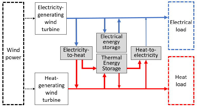
Figure 1.7: Possible energy conversion steps and storage components from wind power
to electricity and heat loads. Blue lines represent electricity and red lines
represent thermal energy. ....................................................................................... 7
Figure 1.5: Energy conversion steps of electricity-generation systems with storage [73].
(A) Non-GIES system with standalone storage. (B) A GIES system. ................... 8
Figure 1.6: Power conversion components in wind turbines for (a) generating electricity
and (b) generating heat. ......................................................................................... 9
Figure 2.1: Power coefficient and blade tip speed curve of different rotor designs [86]. ....... 13
Figure 2.2: Rotational speeds, wind turbine radius, and torque of wind turbines with
different power capacities, based on the data in [81]. ......................................... 14
Figure 2.3: Different wind-powered thermal systems configured with different wind-
driven heating technologies for space heating [57]. ............................................ 15
Figure 2.4: The component and cost breakdown of a 2 MW wind turbine [120]. .................. 22
Figure 2.5: An example of the generation of eddy currents on spinning circular disk
[125]. .................................................................................................................... 23
Figure 2.6: The structure of an eddy current heating device for drying powders and grains
[61]. ...................................................................................................................... 24
Figure 2.9: A typical structure of eddy current heaters [63]. .................................................. 25
Figure 2.7: The illustrations of an outer rotor permanent magnet eddy current heater [62]:
a) an outer, b) an inner stator, and c) a vertical axis wind turbine that the hub
is directly mounted on the outer rotor. ................................................................. 26
Figure 2.8: A two-dimensional schematic of the generation of eddy currents in a
conductor. (a) Magnetic poles and a cylindrical conductor. (b) Traveling-
wave approximation [70]. .................................................................................... 27
Figure 2.10: The structure of an eddy current heater with inner conducting rotor [69]. ......... 31
Figure 2.11: Thermal power of eddy current heater with different numbers of magnet
poles in three studies: (a) Fireteanu and Nebi [63] at 1,000 RPM; (b)
Tudorache and Popescu [64] at 400 RPM with 30 mm thickness of steel; (c)
Tudorache et al. [60] at 180 RPM with 10 mm thickness of magnetic steel. ...... 33
ix
Figure 2.12: Thermal power against conductor thickness in different studies: (a) Nebi
and Fireteanu [63] at 1,000 RPM with steel conductor; (b) Tudorache and
Popescu [64] at 400 RPM with steel conductor. .................................................. 34
Figure 2.13: Thermal power of the eddy current heaters with different conducting
materials: (a) stainless steel and (b) aluminium [61]. .......................................... 34
Figure 2.14: Thermal power of the eddy current heater with different materials as
conductor (AL: aluminium, CO: copper, ST: steel), conductor thickness 30
mm and 400 RPM [64]. ....................................................................................... 35
Figure 2.15: Rotational speed vs. skin depth with n=4 (number of magnet poles). ................ 36
Figure 2.16: Illustration of the air gap in a quarter of typical eddy current heater structure
with sectional view. ............................................................................................. 37
Figure 2.17: Tudorache and Popescu [64] at 400 RPM, steel as conductor, 30 mm
conductor thickness. ............................................................................................ 37
Figure 2.18: The required temperature for different industrial processes and the
maximum heating temperature of low-carbon energy sources [177]. ................. 45
Figure 2.19: Air temperatures and COP of air-source heat pumps (EXT_AIR; light green)
and heat pumps coupled with earth-to-air heat exchanger (EAHX) at the
coldest days in three different cities [181]. .......................................................... 47
Figure 2.20: The transmission distance and transmission capacity of different
transmission technologies, such as high voltage direct current (HVDC), high
voltage alternative current (HVAC) and heat transmission pipelines [134]. ....... 50
Figure 2.21: Thermochemical storage with decoupled power and storage capacity [191].
............................................................................................................................. 51
Figure 2.22: The UK’s daily average of electricity demand, wind and solar generation,
and day-ahead market price in 2019 [29] [196]. .................................................. 53
Figure 3.1: The sensitivity of the design factor and the power of rotational speed
to the thermal power of eddy current heaters, based on rotational speed
at 200 RPM. ......................................................................................................... 62
Figure 3.2: Conducting cylinder temperature against the factor of pipeline length from
one to five with different HTFs (i.e. water, mineral oil, and air) and heat
transfer coefficient. .............................................................................................. 66
Figure 3.3: Sectional view of the proof-of-concept eddy current heater. ................................ 68
Figure 3.4: The HTF inlet (blue) and outlet (red) channels on the cover plate (left) and
the HTF distribution channels on the front plate (right). ..................................... 69
Figure 3.5: The illustration of a two-layer flow path in the proof-of-concept eddy current
heater. A HTF is introduced into the heater in the inner layer and returned
from the outer layer. ............................................................................................ 69
Figure 3.6: Heat transfer diagram of the proof-of-concept heater, with four heat transfer
directions (shown by arrows with numbers) and six surfaces that have heat
loss to the environment (red solid arrows). ......................................................... 71
x
Figure 3.7: Thermal resistance of the eddy current heater. ..................................................... 71
Figure 3.8: Proposed experimental setup for the eddy current heater. .................................... 75
Figure 3.9: The magnet setup for the preliminary tests. The number of magnet poles is
16. ........................................................................................................................ 76
Figure 3.10: Experimental setup for the preliminary tests. ..................................................... 77
Figure 3.11: Experimental setup without partition between the motor and the heater............ 77
Figure 3.12: Diagram of the location of thermocouples TC 1 to TC 9 for the preliminary
tests. ..................................................................................................................... 78
Figure 3.13: Temperature profile of each component in starting and heating phase. ............. 80
Figure 3.14: Rate of temperature change in starting and heating phases. .............................. 81
Figure 3.15: Temperature profile after heater after heater is stopped. .................................... 82
Figure 3.16: Rate of temperature change after heater is stopped. ........................................... 83
Figure 3.17: Average thermal power vs. estimated rotational speed. ..................................... 84
Figure 3.18: Calculated heat loss in constant frequency tests: (a) 40 Hz, (b) 35 Hz, (c) 30
Hz, and (d) 20 Hz. ................................................................................................ 85
Figure 3.19: An illustration of heat loss to the baseplate through the front and rear plates.
Deep blue represents low temperature, and yellow and green represents
higher temperature. The temperature at the feet of front and rear plates are
lower than other parts of the heater. .................................................................... 86
Figure 3.20: Temperature profile for the core temperature measurement............................... 87
Figure 3.21: Illustration of heaters with and without thermal insulation between the
front/rear plates and conducting/outer cylinders. Red, yellow, and blue
colour represent high, medium, and low temperature, respectively. ................... 90
Figure 3.22: The coupling between the heater and the motor by hubs and coupling torque
disk. ...................................................................................................................... 91
Figure 3.23: (a) chipped magnets, (b) a screw got loose on the core, (c) a damaged heater
shaft and (d) failed rear bearing ........................................................................... 92
Figure 4.1: A load duration curve against a residual load duration curve [233]. .................... 96
Figure 4.2: Residual load duration curves with different VRE shares, based on 2018
electricity data for the UK [29]; seasons are shown in different colours. ........... 97
Figure 4.3: Wind generation in different residual load bands. ................................................ 98
Figure 4.4: Simulation of variable renewable energy with energy storage. ............................ 99
Figure 4.5: System configurations of five wind power systems integrated with electrical
energy storage or thermal energy storage. ......................................................... 101
Figure 4.6: 2016 UK wind power data. ................................................................................. 105
Figure 4.7: Schematic of wind power systems includes all components. ............................. 105
Figure 4.8: Example of base load in a one-week operation, during January 17–23, 2016.... 109
xi
Figure 4.9: Base load with different system output targets. .................................................. 109
Figure 4.10: One-week system output profile for peaking power, during January 21–27,
2016. .................................................................................................................. 110
Figure 4.11: One-week system operation for output firming, during January 1–7, 2016. .... 111
Figure 4.12: Annual output profiles of system 2 for the base load scenario with storage
durations of (a) no storage, (b) 10 hours and (c) 20 hours. ............................... 113
Figure 4.13: LCOE, charging and rejection rate, and average output of systems 1 to 5
with storage durations of 0 to 30 hours for the base load scenario. ................... 114
Figure 4.14: Output profile of system 1 for peaking power in a high-wind-power week
with different storage durations of (a) 5 hours, (b) 10 hours and (c) 15 hours.
........................................................................................................................... 117
Figure 4.15: LCOE, charging and rejection rate and average output of systems 1, 2, 3 and
5 with storage durations of 0 to 15 hours for the peaking power scenario. ....... 118
Figure 4.16: One-month (January 2016) output profile of system 4 for output firming
with storage durations of (a) no storage, (b) 3 hours and (c) 9 hours. Note
that ‘hWT to TES’ is the thermal power charging into TES and ‘hWT to
grid’ is electric power supplied to the grid. ....................................................... 120
Figure 4.17: Box plots of system output at the minimum, 5th, 25th, 50th, 75th, 95th and
maximum percentiles. ........................................................................................ 121
Figure 4.18: LCOE, charge percentage and average output power for the output firming
scenario. ............................................................................................................. 123
Figure 4.19: System output boxplots of system 1, 2, 4 ( 0.2 and 0.3) and 5 (
0.1 and 0.2) for output firming scenario at a system cost of 80 £/MWh. The
boxplot on the left (Ref.) is a reference system without energy storage. .......... 124
Figure 4.20: Energy flow of systems 1, 2, 4 ( 0.2) and 5 ( 0.1) at a reference
cost of 80 £/MWh for the output firming scenario. ........................................... 125
Figure 4.21: Sensitivity analysis for the base load scenario. ................................................. 127
Figure 4.22: Sensitivity analysis for the peaking power scenario. ........................................ 128
Figure 4.23: LCOE of WTES and non-GIES at different charge percentages for
sensitivity analysis, i.e. capital cost of heat-generating wind turbine (hWT),
capital cost of electricity-to-heat component (E2H) and heat-to-electricity
efficiency. .......................................................................................................... 129
Figure 5.1: Normalised wind and solar generation and space heating demand in (a) a
week (January 2–8) [29], [245], [246]. .............................................................. 137
Figure 5.2: Normalised wind and solar generation and space heating demand in a year in
the UK, 2019 [29], [245], [246]. ........................................................................ 137
Figure 5.3: Heat demand profiles with different baseload heating fractions (0, 25, 50, 75
and 100%), with annual heat demand of 10 GWh. The baseload heating
fraction is defined as the fraction of baseload heating demand over total heat
demand, which is the summation of baseload and space heating demands. ...... 138
xii
Figure 5.4: The results of (a) the profile of wind power for space heating, (b) the profile
of solar energy for space heating, and (c) the profile of wind power for
demand profile with baseload heating fraction of 0.7, and (d) storage
capacity and percentage with different baseload heating fractions. Based on
the UK’s wind, solar, and space heating demand profiles in 2019. ................... 139
Figure 5.5: Possible energy conversion routes from wind power to heat users. ................... 141
Figure 5.6: Proposed wind-powered thermal energy system configuration for district
heating. ............................................................................................................... 151
Figure 5.7: The profiles of heat demand and operation of heat storage for district heating
with 10 GWh of annual heat demand, based on storage efficiency of 70%. ..... 152
Figure 5.8: Levelised cost of storage of heat storage with 0.3, 0.5 and 0.8 £/kWh of
capital cost, storage efficiency 50, 70 and 90%, and lifetime 20, 30, 40 and
50 years; based on the discount rate of 7% and O&M costs is 0.7% of the
capital cost. ........................................................................................................ 154
Figure 5.9: LCOE of WTES for district heating with different wind-driven heating
technologies (i.e. electric boilers and mechanical heat pumps) and wind
power capacity factor (0.15–0.3); blue lines present the results from [57]
(without seasonal storage); orange lines present the LCOE with seasonal
storage (storage efficiency 70%; capital cost 0.5 £/MWh). ............................... 154
Figure 5.10: The correlation between increasing wind turbine capacity and (a) the
reduction of storage capacity and (b) ratio of storage capacity to wind turbine
capacity; with storage efficiency of 50%, 70% and 90%. ................................. 155
Figure A.1: Radiation heat transfer between two long concentric cylinders [268]. .............. 161
Figure A.2: Radiation heat transfer rate at the air gap with different surface temperature
and emissivity (i.e. 0.1, 0.5 and 0.8), based on the dimension of the proof-
of-concept heater. .............................................................................................. 162
Figure A.3: 3D drawing of the proof-of-concept eddy current heater. ................................. 163
Figure A.4: Temperature profile of each thermocouple before calibration. .......................... 166
Figure A.5: The illustration of (a) the temperature of gap filler () is estimated from
temperature reading of thermocouple TC 2 (), and (b) The energy
balance on a volume element cut out from a cylinder [274]. ............................ 168
Figure A.6: Experimental results of 40Hz test without stop for thermal power estimation.
........................................................................................................................... 171
Figure A.7: Experiment results of 40 Hz test without stop for heat loss estimation. ............ 172
Figure A.8: Experiment results of 35 Hz test without stops for heat loss estimation.
Temperature of the front port (TC1) has a peak at 18 min due to the friction
of coupling and cover plate after the coupling got loose. Several data
recording interruption after 1 hour 50 min due to the unstable connection
between the data logger and recording software. .............................................. 173
xiii
Figure A.9: Experiment results of 30Hz test for heat loss estimation. Several data
collection interruption at 45 min and 1 hour 10 min due to the unstable
connection to the data logger and software. ...................................................... 174
Figure A.10: Experiment results of 20 Hz test for heat loss estimation. The ambient
temperature was dropped at 5 hour due to the main door of lab was open for
few minutes. ....................................................................................................... 175
Figure A.11: The temperature readings and calculated temperature of the gap filler in the
heating phase of constant frequency tests. The temperature of gap filler was
3.1°C, 2.3°C, 1.3°C and 0.4°C higher than the temperature of TC 2 in the
test of 40, 35, 30 and 20 Hz, respectively. ......................................................... 176
Figure A.12: Electric motor part-load efficiency (as a function of full-load efficiency)
[276]. .................................................................................................................. 177
Figure A.13: Experiment results of 40 Hz test with stops at TC 2 at 25, 35, 45 and 55°C.
........................................................................................................................... 178
Figure A.14: Experiment results of 30 Hz test with stops at TC2 at 25, 35, 45 and 55°C. ... 179
Figure B.1: Algorithm of searching output target for output smoothing. ............................. 182
Figure B.2: Example of searching system output target for capacity firming....................... 183
Figure C.1: the hydrogen pipeline cost with different outer diameter and sources [251]. .... 185
Figure C.2: the cost of compressed gas storage for hydrogen storage [252]. ....................... 185
Figure C.3: Dehydration of calcium hydroxide of a 10-MW reactor [165]. ......................... 186
Figure C.4: Hydration of calcium oxide in a 10-MW fluidised bed reactor. ....................... 187
xiv
LIST OF TABLES
Table 2.1: Selected patents related to wind-driven heating technology. ................................. 17
Table 2.2: A summary table of technologies for converting kinetic energy to heat from
literature. .............................................................................................................. 18
Table 2.3: The properties of selected heat transfer fluid. ........................................................ 21
Table 2.4: Design factors of an eddy current heater [61]. ....................................................... 25
Table 2.5: Summary of correlations between thermal power and design parameters. ............ 29
Table 2.6: The properties of four common permanent magnets [130]. ................................... 32
Table 2.7: The properties of common conducting materials [131][132]. ................................ 35
Table 2.8: Properties of common solid sensible heat storage materials [138]. ....................... 39
Table 2.9: Properties of liquid sensible heat storage materials [139]. ..................................... 39
Table 2.10: Parameters of large-scale sensible heat storage systems [141], [142]. ................. 40
Table 2.11: Properties of common phase change material [139], [147]. ................................. 41
Table 2.12: Chemical reactions for TCS [156]. ....................................................................... 42
Table 2.13: Sorption processes for TCS [155]. ....................................................................... 43
Table 2.14: The density and volumetric energy density of hydrogen with low heating
value (LHV, 33.3 kWh/kg) at different conditions [185]. The high heating
value (HHV) of hydrogen is 39.4 kWh/kg. ......................................................... 49
Table 2.15: Operational parameters of energy storage systems for different services
[197]. .................................................................................................................... 54
Table 2.16: Typical round-trip efficiency and energy-power ratio of different energy
storage technologies [45], [199]. ......................................................................... 54
Table 3.1: The parameters of 10 kW, 250 kW and 6 MW representative wind turbines. ....... 60
Table 3.2: The summary of design parameters of eddy current heaters from different
studies. * is the results from experimental studies. Others are the results from
FEM simulation. .................................................................................................. 62
Table 3.3: Estimated size of 10 kW and 6 MW eddy current heaters. .................................... 63
Table 3.4: Heat transfer parameters of selected HTFs for a 10 kW eddy current heater. ....... 64
Table 3.5: The temperature of each component. ..................................................................... 79
Table 3.6: Experimental result of the continuous heating test. ............................................... 84
Table 4.1: Efficiency parameters of energy storage and secondary energy converters that
used in the analysis in this chapter. ................................................................... 102
Table 4.2: Cost parameters of components based on the projection for 2025. ...................... 103
Table 4.3: The results of each system with lowest LCOE for the base load operation. ........ 115
xv
Table 4.4: The results of each system with lowest LCOE for the peaking power operation.
The average output power is calculated in peak hours only (5 hours in a day).
........................................................................................................................... 119
Table 4.5: Sensitivity analysis parameters............................................................................. 126
Table 4.6: The component efficiency and capital cost for each system. ............................... 130
Table 5.1: The components in four wind-to-heat routes........................................................ 141
Table 5.2: The cost parameters of the components of each wind-to-heat route. ................... 143
Table 5.3: the energy loss in each part of routes. .................................................................. 146
Table 5.4: Summary of the comparison of system flexibility, cost and efficiency of each
route; ‘+’ for advantage and ‘-’ disadvantage. ................................................... 150
Table 5.5: System parameters for district heating. ................................................................ 153
Table A.1: The emissivity of common metals and surfaces [269]. ....................................... 162
Table A.2: Material properties and specification of each component. .................................. 164
Table A.3: Thermal resistance for heat loss calculation. ....................................................... 165
Table A.4: Thermal resistance for the heat transfer in the radial direction. .......................... 165
Table A.5: Thermal resistance for the heat transfer in the axial direction. ........................... 166
Table A.6: Thermocouple calibration data, before calibration. ............................................. 167
Table A.7: Specification of Variable Frequency Drive (VFD) [271]. ................................... 167
Table A.8: 1.5 kW Single-Phase AC motor [272]. ................................................................ 167
Table A.9: Calcium-Magnesium Silicate thermal insulation sheet [273].............................. 167
Table A.10: Material cost of the proof-of-concept eddy current heater. ............................... 180
Table A.11: Material properties of the proof-of-concept eddy current heater [131]. ............ 180
Table A.12: Properties of permeant magnets [277]. .............................................................. 180
Table C.1: The range of maximum temperature for process heating in different industries
[278]. .................................................................................................................. 184
Table C.2: Solid-gas thermochemical storage candidates [164]. .......................................... 184
i
NOMENCLATURE
Area (m
2
)
Amplitude of the traveling wave (T)
Strength of magnetic field (T)
Specific heat of component (J/kg.K)
Specific heat capacity of a material (J/kg.K)
Capital cost of component (£)
Operational cost of component (£)
Power coefficient of wind turbines
Total cost of system in year (£)
Diameter of pipeline (m)
Stored energy at time (MWh)
Total produced energy in year (MWh)
Rotational speed (Hz)
Mass flow rate of HTF (kg/s)
Air gap thickness (m)
Heat transfer coefficient (W/m
2
.K)
Heat of fusion/evaporation per unit mass (J/m
3
)
Reaction enthalpy or heat of sorption for TCS (kJ/mol)
Thermal conductivity of a material (W/m.K)
Length of conducting cylinder (m)
Length of an object or component (m)
Mass of an object or component (kg)
Fundamental wave amplitude of the residual magnetisation intensity
Lifetime of a system or component (year)
Rotational speed (RPM)
Number of magnetic pole pairs
Power of a component or a system (W)
Available wind power extracted by wind turbines (W)
ii
Power of a rotational machine (W)
Thermal power of a heat generator (W)
Heat transfer rate (W)
Latent heat (J)
Sensible heat (J)
Radius of a wind turbine (m)
Radius of conducting cylinder (m)
Discount rate (%)
Thermal resistance of a material (K/W)
Time (second or hour)
Temperature (K)
Logarithmic mean temperature difference (K)
Internal energy (J)
Velocity of a fluid (m/s)
Volume of conducting cylinder (m
3
)
Rotational work (W)
Design factor of an eddy current heater
Fraction of phase change (%)
Fraction of hWT in a wind power system
Number of year of a project or system (year)
Power of rotational speed of an eddy current heater
Greek Symbols
Arc length coefficient
Effective skin depth (m)
Emissivity of a material
Energy conversion efficiency (%)
Tip speed ratio of a wind turbine
Permeability of a material (H/m)
Vacuum permeability (H/m)
Relative permeability of a material
iii
Density of a material (kg/m
3
)
Conductivity of a material (S/m)
Torque (Nm)
Abbreviations
AC
Alternating Current
AlNiCo
Aluminium Nickel Cobalt
ATES
Aquifer Thermal Energy Storage
BOS
Balance of System
BTES
Borehole Thermal Energy Storage
CAES
Compressed Air Energy Storage
CAGR
Compound Annual Growth Rate
CCS
Carbon Capture and Storage
CHP
Combined Heat and Power
COP
Coefficient of Performance
CSP
Concentrating Solar Power
DC
Direct Current
DSM
Demand Side Management
E/P ratio
Energy-Power Ratio
E2H
Electricity-to-heat
EES
Electrical Energy Storage
ES
Energy Storage
eWT
Electricity-generating Wind Turbine
FEM
Finite Element Method
FM
Fluidisation Medium
GIES
Generation-Integrated Energy Storage
H2E
Heat-to-Electricity
HAWT
Horizontal Axis Wind Turbine
HHV
Higher Heating Value
HP
High Pressure
HTF
Heat Transfer Fluid
iv
hWT
Heat-generating Wind Turbine
ID
Inner Diameter
LAES
Liquid Air Energy Storage
LCOE
Levelised Cost Of Energy
LCOS
Levelised Cost Of Storage
LHV
Lower Heating Value
NdFeB
Neodymium-iron-boron
NPV
Net Present Value
O&M
Operations and Maintenance
OD
Outer Diameter
ORC
Organic Rankine Cycle
PCM
Phase Change Material
PitTES
Pit Thermal Energy Storage
PTES
Pumped Thermal Electricity Storage
PV
Photovoltaic
RLDC
Residual Load Duration Curve
RPM
Revolutions Per Minute
SmCo
Samarium–cobalt
STP
Standard Temperature and Pressure
TC
Thermocouple
TCS
Thermochemical Storage
TES
Thermal Energy Storage
TEU
Twenty-foot Equivalent Unit
TRL
Technology Readiness Level
TTES
Tank Thermal Energy Storage
V2G
Vehicle-To-Grid
VFD
Variable-Frequency Drive
VRE
Variable Renewable Energy
WT
Wind Turbine
WTES
Wind-powered Thermal Energy System
v
PUBLICATIONS AND PRESENTATIONS
Publications
Y. C. Chen, J. Radcliffe, and Y. Ding, “Concept of offshore direct wind-to-heat system
integrated with thermal energy storage for decarbonising heating,” in 2019 Offshore Energy
and Storage Summit (OSES), 2019, pp. 1–8.
Reports
J. Radcliffe, J. Greaves, R. Heap, Y. C. Chen, “Immediate need for substantial investment in
energy storage”, Energy Research Partnership, September 2020
“Innovation Outlook: Thermal Energy Storage”, IRENA October 2020 (report contributor)
Presentations
“Assessments of Wind powered Thermal Energy System for heat & power supply”, 2nd
German-Japanese Workshop on Renewable Energies, Stuttgart, Germany, July 2017
“The value of thermal energy storage in decarbonizing the electricity industry”, UK Energy
Storage Conference, Newcastle, UK, March 2018
“Thermal energy storage research projects in the University of Birmingham”, IEA ECES Annex
on Carnot Batteries Workshop, Stuttgart, Germany, May 2019
Posters
“Assessments of Wind powered Thermal Energy System (WTES) for base load generation”,
UK Energy Storage Conference, Newcastle, UK, March 2018
“Direct wind-to-heat system with high-temperature thermal energy storage for decarbonising
heating”, UK Energy Storage Conference, Newcastle, UK, September 2019
1
1 INTRODUCTION
1.1 Background
1.1.1 Wind power in low-carbon energy systems
Human activities are extremely likely to have been the primary cause of global warming. Global
temperatures have increased approximately 1.0°C above pre-industrial levels and are likely to
reach 1.5°C before the middle of this century if the increase rate is not changed [1]. Many
countries have pledged net-zero carbon emissions to mitigate climate change [2], [3]. In 2020,
six countries set their targets in national legislation (i.e. Sweden, United Kingdom, France,
Denmark, New Zealand, and Hungary), four are in the process of legislating (i.e. EU, Spain,
Chile, and Fiji), and many are under discussion or in policy documents.
In the past ten years, the carbon emission of some countries has fallen by increasing the share
of renewable energy in their electrical energy systems. However, the fluctuating generation
from Variable Renewable Energy (VRE) sources may cause the electric system to be unstable
and unreliable. In order to maintain a stable electrical grid, various technologies have been
studied and developed to provide flexibility to electrical energy systems, such as Demand-Side
Management (DSM) [4], [5], interconnections to neighbouring electrical networks [6], [7], and
integration of energy storage [8]–[10]. In order to achieve deep decarbonisation or net-zero
targets, the greenhouse gas emissions in all sectors (e.g. power generation, industry, buildings,
and transport) need to be cut down significantly [11]. However, decarbonising some of the
energy sectors are challenging due to their unique characteristics, such as high energy density
(e.g. aviation [12]), high peak demand and significant seasonal demand variations (e.g. space
heating [13]). Technology innovation is needed to accelerate the transition to low-carbon
energy systems.
Wind power is one of the most abundant renewable energy sources in the world. The energy
cost of wind power is continuously decreasing and could be the cheapest electricity generation
source by 2030 [14]. At the end of 2018, global wind power installed capacity reached 597 GW,
supplying nearly 5% of the worldwide electricity demand [15]. However, the current installed
capacity is still far less than the global wind power potential, which could be over 200,000 GW
[16]. Wind power plays a vital role in the future energy system in the UK. Cavazzi and Dutton

2
[17] estimated the economically accessible offshore wind power in the UK is 675 GW or over
2,600 TWh of wind energy in a year, which is much more than the estimated total annual energy
consumption (600–900 TWh) of net-zero scenarios in 2050 [18], [19]. Figure 1.1 shows the
power capacity of non-dispatchable low-carbon energy sources (i.e. wind, solar PV and nuclear)
in different net-zero scenarios. The installed capacity of wind power is expected to increase
substantially from 22 GW in 2019 to 55–130 GW in 2050. The penetration of VRE (i.e. wind
and solar) is expected to increase from 25% to over 67%. High VRE penetration in an electrical
energy system means that a significant amount of dispatchable generation and flexible energy
management systems is needed to balance the grid.
Figure 1.1: UK’s electricity generation forecast to 2030 and 2050 [18], [19].
1.1.2 Intermittency of wind power
Wind power can be variable over different timescales from milliseconds [20] to months [21].
Low or high-wind periods typically may last hours to a few days (see Figure 1.2). There are
also seasonal variation patterns, with the wind speed in winter usually being higher than in
summer. Figure 1.3 shows the UK’s monthly average capacity factor of wind power in 1980–
2016 [22]–[24]. It can be observed that the average capacity factor in winter is generally higher
than in summer, and the year-to-year variation in winter is higher than in summer. The median
capacity factor in January is 0.46, but it could be lower than 0.3 or higher than 0.6 some years.
Various wind power forecast methods for different time scales such as minutes ahead, hours

3
ahead, weeks ahead and years ahead were developed [25], [26]. Accurate wind generation
prediction can reduce the total electricity generation cost in energy systems by minimising the
reserve power and reducing the uncertainty in electricity markets [27]. However, deploying
systems that can balance wind power generation and energy demand over different time scales
are necessary [8], especially for a country or region that has high wind power penetration in
their electrical energy systems, such as Denmark (41%), Ireland (28%), and Portugal (24%) in
2018 [28].
Figure 1.2: UK wind power generation on January and July, 2019 [29].
Figure 1.3: Estimated monthly average capacity factors of wind power in the UK, based on
historical weather data in 1980–2016 and present-day fleet of wind farm for both onshore and
offshore wind farms [22]–[24].
4
1.1.3 Solutions to balance energy supply and demand
Each electric power system normally has a certain amount of flexible power to follow demand
changes in a day, a week and different seasons. If the share of VRE generation in an electrical
system is low such as less than 10%, this existing flexible power generation units are usually
enough to maintain grid stability. However, when the penetration is high such as over 20-40%,
integrating VRE generation to electrical grids can pose challenges for grid operators [30]–[32].
The intermittency of wind generation can reduce the power quality and reliability of the system
and increases the requirement for reserve power. Upgrading transmission systems is needed to
avoid grid congestion. Several technologies were studied to balance the electric power grid and
enhance the flexibility of electrical energy systems [33], [34], such as flexible generation
sources, DSM, grid interconnection and energy storage.
Power plants that have short start-ups and fast ramping rates (e.g. hydropower and gas turbine
power plants) can quickly adjust their output with changing electricity demand and generation
from VRE sources [35]–[37]. However, installing flexible power plants has several limitations.
Hydropower can only be installed in the locations with specific geographical conditions, such
as mountainous regions with water sources. Conventional gas-fired power plants emit carbon
dioxide while generating power. This emissions can be reduced by carbon capture and storage
(CCS) [38] or the use of hydrogen gas turbines [39], [40], but both technologies require high
investment costs and long installation time.
DSM changes the energy demand by influencing the behaviour of energy consumers [41], [42].
DSM could reduce the demand at peak hours and shift it to another time, thereby reducing the
need for backup power. However, DSM can only provide a certain level of demand shift and is
not able to resolve the issues over long periods of time, such as low-wind periods which last
several consecutive days and balancing seasonal demand variations.
Interconnection between neighbouring power grids enables power exchanges. This allows the
export of excess VRE generation to avoid curtailment and the import of electricity to reduce
the use of backup power plants [6]. As a result, interconnection can not only reduce carbon
emissions but also lower the average value and variation of electricity prices [43]. However,
building interconnection lines requires high investment costs and long planning and
construction times (e.g. the construction time for the interconnector between Great Britain and
European countries is about 4 to 6 years [44]). The benefits of connecting electrical grids are
5
limited if the connected electrical systems have similar energy mixes and renewable energy
generation profiles.
Energy storage is the capture of energy for later use. Energy can be stored in different forms,
such as electrical, chemical, mechanical and thermal energy [45]. Integrating energy storage to
electrical grids could decouple VRE generation and electricity demand [46], thereby avoiding
energy curtailment. However, a part of the stored energy will be lost between charge and
discharge processes. Energy storage can provide flexibility to an energy system on time scales
from short-term (e.g. milliseconds) to very long-term (e.g. months or years) [46], [47]. An
energy storage system can be integrated at different levels of electrical grids, i.e. generation,
grid operation and customers [48]. On the generation side, integrating energy storage with
power generation systems can potentially increase the revenue of the system by price arbitrage
[49] and improve the utilisation of transmission lines by congestion management [50]. For grid
operation, energy storage can provide different grid services such as frequency response [51],
load-levelling [52] and operating reserves [52]. Installing behind-the-meter energy storage
systems on the consumer side can provide various applications such as on-site backup power,
storage for off-grid VRE generation, and load shifting [53]. The energy storage devices on the
customer side can also provide grid services if a large number of devices are gathered together,
such as Vehicle-to-Grid (V2G) [54].
1.2 Direct wind-to-heat energy systems
1.2.1 A new way to use wind power
A direct wind-to-heat system converts wind power to heat at the generation side and stores that
heat in thermal energy storage for later use. This system is also called a Wind-powered Thermal
Energy System (WTES) [56]. In principle, WTES has a minimal number of energy conversion
steps to convert wind power into heat, and the investment cost and energy loss of the system
are therefore lower than those of other systems, such as a conventional wind power system that
converts wind power to electricity and then generates heat by electric heaters.
The concept of WTES was first proposed by Okazaki et al. [56] for baseload power generation
(see Figure 1.4). The generated heat is stored in high-temperature heat storage such as molten
salt storage, and the stored heat is converted into electricity by steam turbines and electric

6
generators. The cost estimation showed that WTES has a cost advantage in long-duration
storage applications over other conventional solutions such as storing wind power in electrical
energy storage. Later, Cao et al. [57] investigated various heat generation technologies for a
WTES that is used for space heating. Different system parameters such as system scales and
capacity factors of wind power were taken into account for cost estimation. The results showed
that the energy cost of WTES could be competitive with other space heating technologies.
Figure 1.4: An example of a wind-powered thermal energy system for power generation [56].
A WTES can be broken down into three parts: wind-to-heat conversion, thermal energy storage
and the use of heat. The function of latter two parts are fundamentally the same as systems
integrated with thermal energy storage. For instance, concentrating solar power (CSP) plants
store heat in thermal energy storage and convert it into electricity [58]. Some district heating
systems store heat from combined heat and power (CHP) plants or solar energy for space
heating [59].
On the other hand, the technology to convert mechanical energy from wind power into heat is
not yet fully explored. Several studies investigated the technology to convert kinetic energy
into heat through modelling [60]–[65] and experimental work [66], [67], but most of these are
aiming for water heating. Technological concepts and device structures to produce high-
temperature heat from kinetic energy through electromagnetic induction were proposed [55],
[56], [68], [69] and studied by theoretical calculation [70]. To the best of the author’s
7
knowledge, there have been no experimental studies of wind-driven heaters for generating high-
temperature heat.
1.2.2 Other wind power systems integrated with energy storage
Conventional systems that convert wind power into electricity can provide the same services as
WTES but require one more energy conversion step to produce heat. Figure 1.5 shows various
energy conversion steps to use wind power to supply electrical or heat loads. For electricity
generation, conventional wind power systems convert wind power into electricity, which can
be stored in electrical energy storage. The generated electricity can also be stored in heat storage
via electrical heating, and the stored heat can be turned back to electricity by heat engines and
electric generators. This type of systems that store electricity in thermal energy storage is also
called Carnot batteries [71], [72]. For heat generation, conventional wind power systems require
an electrical heating component to produce heat.
Figure 1.5: Possible energy conversion steps and storage components from wind power to
electricity and heat loads. Blue lines represent electricity and red lines represent thermal energy.
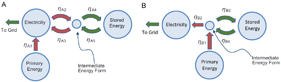
Generation-integrated energy storage
In the context of energy storage systems, WTES can be considered as a generation-integrated
energy storage (GIES) system, which converts and stores primary energy in an intermediate
form and then converts the stored energy into electricity upon demand [73]. Figure 1.6
illustrates the energy conversion routes of non-GIES and GIES systems. GIES systems need
8
one more energy conversion step to produce electricity but have fewer energy conversion steps
as energy passes through energy storage. Therefore, GIES systems are in principle suitable for
applications in which a high fraction of generated energy needs to be stored for later use. Several
technologies can be classified as GIES, such as CSP and a wind-driven pumped heat thermal
energy storage system [74]. The costs of a GIES system that integrates wind turbines and
pumped thermal energy storage were estimated and compared with other solutions for a grid
balancing problem with different charging and discharging cycle times [75]. The results showed
that this GIES system has lower annual costs when the cycle time is longer than five hours.
Moreover, the system has a higher efficiency than standalone energy storage whilst a high
fraction of energy passes through storage.
The energy costs of different configurations for WTES were estimated in [56], [57], but those
costs are calculated without considering wind power profiles. Unlike standalone energy storage
systems, the input power to a GIES system is determined by its generation units, and it cannot
be controlled if the system is powered by a VRE source such as wind power or solar energy.
Therefore, the profile of power input to GIES systems needs to be taken into account whilst
designing the system and estimating its energy cost.
Figure 1.6: Energy conversion steps of electricity-generation systems with storage [73]. (A)
Non-GIES system with standalone storage. (B) A GIES system.
1.2.3 Wind-driven heat generator
WTES and conventional wind power systems convert wind power into different forms of
energy. Figure 1.7 shows the conversion components in wind turbines that generate electricity
or heat. For electricity-generating wind turbines (see Figure 1.7a), the kinetic energy extracted
from wind power is converted into electrical power by electric generators. Power converters

9
and transformers modify the properties of electrical power such as voltage and frequency to
match the specification of electrical grids [76]. About 5–10% of the energy is lost as heat in the
conversion from kinetic energy to electric power, including the energy loss in generators and
gearboxes [77]. Most large-scale onshore wind turbines are equipped with gearboxes to alter
the low rotational speed from wind turbine blades (e.g. 10–15 RPM) to a higher speed (e.g.
1,500 RPM) that is suitable for the operation of electric generators. However, the gearbox is
expensive (6–12% of the total cost of a wind turbine [78]), accounts for about 1% output loss
[77] and has the highest failure rate and downtime among wind turbine components [79].
A wind turbine equipped with direct-drive electric generators do not need a gearbox. Direct-
drive electric generators can operate at a low rotational speed by increasing the space for
magnetic induction, but this type of generator has higher capital costs and a large size [80].
Direct-drive generators are widely equipped on offshore wind turbines to lower the maintenance
requirements, although direct-drive generators are 2–8 times heavier than geared generators
[78].
Figure 1.7: Power conversion components in wind turbines for (a) generating electricity and
(b) generating heat.
Figure 1.7b illustrates a heat-generating wind turbine that is equipped with a heat generator to
convert kinetic energy into heat and transfer the heat by a fluid. An estimation suggested that
the weight of a heat generator can be only one-tenth that of a direct-drive generator [56]. In
theory, this turbine has nearly no energy conversion loss in the generator because all kinetic
10
energy is eventually turned into heat. However, heat could be lost to the environment in the
generation and transmission systems, especially when high-temperature heat is produced.
Furthermore, auxiliary components such as heat transfer pumps are needed to carry the
generated heat to storage or generation units, and these auxiliary components consume energy.
Further investigation is needed to evaluate the cost and efficiency of this type of generation
system.
In summary, a wind-driven heat generator should have the following features: high power
density that the generator has less weight or volume than conventional generators; high drag
force that the generator can operate at low rotational speeds and therefore no need to equip a
gearbox; low energy losses and low auxiliary energy consumption that enable a high energy
conversion efficiency.
1.3 Aim and objectives
The aim of this research is to investigate the technical feasibility and economic viability of
direct wind-to-heat energy systems. This work can be divided into two parts: the technical
assessment of a wind-driven heating technology for high-temperature heat generation, and the
economic assessment of direct wind-to-heat system for electricity and heat generation.
The ultimate objective of the technical assessment is to construct a wind-driven heater for
generating high-temperature heat and to find out the correlation between design parameters and
device performance by experimental studies. The outcome will help to estimate the device
performance and limitation of the wind-driven heating technology.
The objective for economic assessment is to develop operational simulation models for direct
wind-to-heat systems by considering wind power and system output profiles, and to estimate
the cost of the system for different applications, such as electricity generation, space heating
and industrial heating. This model will help to understand the potential role of direct wind-to-
heat systems in a low-carbon energy system.
1.4 The structure of this thesis
In chapter 2, existing studies within the scope of direct wind-to-heat systems are reviewed to
provide a background to the whole thesis. This involves comprehensive reviews of wind-to-
11
heat systems and technologies, studies on eddy current heaters, thermal energy storage
technologies and their integration with wind power, and the heating technologies using wind
power as the energy source, and the economic assessment of energy generation and storage
systems.
The aim of chapter 3 is to understand the potential performance and limitations of wind-driven
eddy current heaters. The design parameters of eddy current heaters are analysed, and a proof-
of-concept device was designed and built for parametric studies. The preliminary test results
are analysed based on the heat generation and transfer models. The design issues and limitations
of this device and this technology are discussed.
The aim of chapter 4 is to evaluate the energy costs of direct wind-to-heat systems for electricity
generation and to compare the energy costs with other benchmark systems. A systematic
framework is developed to simulate the operation of each system under different operational
scenarios with the consideration of variable generation profiles and the parameters of energy
conversion and storage components. The costs of WTES are compared with other systems that
also integrate wind turbines with energy storage.
The aim of chapter 5 is to understand the potential system benefits of using WTES for heating
applications. The investment costs and energy conversion efficiency of WTES for heat
generation are discussed and compared with other wind-to-heat systems. The system
parameters and costs of WTES for district heating were investigated in a case study, and the
energy costs are compared with other low-carbon heating sources.
In chapter 6, the key findings and results of this work are summarised. Conclusions and future
research areas are given at the end.

12
2 LITERATURE REVIEW
2.1 Wind-to-heat energy systems
2.1.1 Characteristics of wind turbines
Wind power has been utilised by humans for centuries [81] and was first used to grind grain or
draw up water [82]. Since the end of the 19th century, wind power started being used for
electricity generation and now accounts for 4.7% of the world’s electricity generation in 2018
[83].
Wind turbines capture wind energy and convert it into mechanical energy on the rotor. The
mechanical energy can be used for various applications such as pumping water and generating
electricity. Many types of wind turbine rotors have been studied [81], e.g. Savonius rotor,
American farm windmill and Dutch windmill. However, today most of the large-scale wind
turbines are aerofoil three-bladed horizontal axis wind turbines (HAWT) which and are easy to
control and have relatively high wind turbine efficiency [84]. HAWT are by far the most
efficient and economical technology to convert wind energy into mechanical energy. The
theoretical maximum efficiency, or Betz limit, is 57.3% [81]. Today’s wind turbines have about
30–45% efficiency and have a peak efficiency of 50% [85].
In a wind power system, an energy conversion component such as mechanical pumps or electric
generators converts the mechanical power from the rotor to another form of energy. Therefore,
the properties of mechanical power from the rotor (e.g. torque and rotational speeds) need to be
taken into account whilst designing the energy conversion component. The characteristics of a
wind turbine can be expressed by the following three equations [81]. Firstly, the power of a
horizontal axis wind turbine can be calculated as
(2.1)
where
is the available power extracted by wind turbines (), is the density of air
(kg/m
3
), is swept area (m
2
), is the velocity of wind (m/s), and
is the power coefficient
of wind turbines. Secondly, the power coefficient of a wind turbine is the function of the tip
speed ratio () of wind turbine blades, which can be expressed by the following equation

13
(2.2)
where
is the rotational speed (RPM) and
is the radius of wind turbine (m). The power
coefficient of a wind turbine has a maximum value at the optimal tip speed ratio, which depends
on the rotor design and the blade design [84] (see Figure 2.1). Thirdly, the power of a rotational
machine (
) can be calculated from torque (, Nm) and rotational speed (
, RPM) which is
given by
(2.3)
Figure 2.1: Power coefficient and blade tip speed curve of different rotor designs [86].
The above equations express the correlation between three key parameters of a wind turbine
generator: the input mechanical power from wind turbines, rotational speeds and the torque
from the rotor. Figure 2.2 illustrates the rotational speed, radius of wind turbines, and torque of
commercial wind turbines at their rated power [81]. As blade length increases, the power of

14
wind turbines increases exponentially, and the rotational speed of wind turbine rotors decreases
linearly to maintain the same tip speed ratio. As a result, the torque on the rotors is higher as
the power of wind turbines increased. Notably, a high-power wind turbine has a low rotational
speed and high torque on the rotor. This correlation needs to be taken into account while
designing the generator of wind turbines.
Figure 2.2: Rotational speeds, wind turbine radius, and torque of wind turbines with different
power capacities, based on the data in [81].
2.1.2 Development of wind-to-heat systems
The design of the device using wind power for heating can be found since the 1970s. James et
al. [87] developed a design procedure for wind-powered heating systems with storage for
domestic heating. In this study, wind turbines were connected to a heating system, and all the
electricity produced from wind power was converted into heat via resistance heating or fluid
dissipation devices. The generated heat was directly delivered to the heating load, and the
excess heat was stored in storage tanks. In this system, wind power was used for heating only
but not directly converted into heat.
The earliest patent on the direct conversion of wind power to heat was issued in 1971 [88]. A
wind-powered pump circulates a fluid in a pipe circuit, and heat is generated in a long coiled
pipe by the friction from the viscous drag forces between the fluid and the pipes. The generated

15
heat is transferred to and stored in a thermally insulated tank through heat exchange between
the pipes. In 1980, a device for generating heat from wind power through eddy current heating
was issued in a patent [89]. An eddy current heating component is immersed in a liquid within
a vessel and coupled with a wind turbine rotor. When the liquid is heated, it can be stored in a
tank and then circulated to the heat loads by a heat transfer fluid.
Cao et al. [57] investigated the cost of wind-powered heating systems configured with different
heating technologies such as resistance heaters, heat pumps and hydrodynamics retarders (see
Figure 2.3). The system has heat storage with the capacity to supply two to ten hours of peak
heat demand. The levelised cost of energy (LCOE) of the systems at different scales such as
households and residential districts was estimated by considering different system parameters
such as wind capacity factor and transmission distance. The results showed that the system
using mechanical heat pumps has the lowest LCOE, and this LCOE is competitive to that of
other heating solutions such as gas boilers and wood chip boilers. However, the integration of
heat storage was not fully investigated. In this study, the energy loss during storage was not
considered, and the wind generation and heat demand profiles were not considered to estimate
the capacity for heat storage.
Figure 2.3: Different wind-powered thermal systems configured with different wind-driven
heating technologies for space heating [57].
Several patents on wind-driven heating devices for low-temperature heating (e.g. water heating)
were published since the 1970s (see Table 2.1), including a heating system that uses wind-
driven heat pumps [90]. A UK-based company founded in 2016 (H2O Turbine Ltd. [91])
developed a wind turbine heating system that can heat water to 90°C by hydraulic heating.
16
However, very few heat-generation wind turbines have been deployed or commercialised, and
the installed capacity is negligible as compared to that of electricity-generating wind turbines
[92]. One of the reasons is that the value of electricity is considerably higher than that of low-
temperature heat. In most of the cases, the price of electricity is at least two times higher than
the price of heat for space or water heating [93], and an electric heat pump can produce two
times or more thermal energy than it consumes [94].
Wind-powered heating system for electricity generation
Wind-powered heating systems that converts and stores wind power as heat and converts the
stored heat into electricity was issued in two patents in 2012 [95], [96]. In this type of system,
a liquid is heated by wind-driven hydrodynamic retarders and is stored in liquid tanks. The heat
stored in the liquid drives organic Rankine cycle (ORC) systems which produce electricity. This
is the first system that was proposed to store wind power in heat storage and produce electricity
upon demand. However, the energy efficiency of this system is limited by the low-temperature
produced by hydraulic retarders and the efficiency of ORC turbines [97]. The concept of a
WTES that generates and stores wind power as high-temperature heat was proposed by Okazaki
et al. [56] in 2015. This system converts wind power into high-temperature heat via
electromagnetic induction machines, and the heat is transferred and stored in high-temperature
thermal energy storage such as molten salts. Steam turbines and electric generators convert the
stored heat into electricity (see Figure 1.4). The energy cost of WTES for base-load operation
is estimated and compared with that of other systems that can also smooth the intermittent
output from wind turbines, such as wind power systems integrated with batteries. A simplified
cost estimation based on fixed capacity factors for each component showed that WTES has the
cost advantage for a long storage duration because of the low cost of thermal energy storage.
With a storage duration of 24 hours, the energy cost of wind power systems integrated with
sodium–sulphur batteries (i.e. 14 JPY/kWh or 102 £/MWh) is considerably higher than the
energy cost of WTES (i.e. 8 JPY/kWh or 58 £/MWh). Different designs to convert wind power
into high-temperature heat through electromagnetic induction have been proposed and filed in
several patents, i.e. induction machines equipped with permanent magnets [68], electric
induction motors for heat generation [55], and superconducting magnetic induction heaters
[69].

17
Table 2.1: Selected patents related to wind-driven heating technology.
Wind-to-heat
Storage
Heat-to-
electricity
Title
Patent number
Publication
date
Hydrodynamic
Liquid
-
Wind motor operated heating system
US3752395 A
8/14/1973
Eddy current
Hot water
storage tank
-
Wind powered heating circuit - has sails on wind tower
driving eddy current brake for producing heat for heat
exchange fluid
DE2901997A1
31/07/1980
Heat pump
-
-
Heat pump operated by wind or other power means
US4304103A
12/08/1981
Hydrodynamic
-
-
Wind driven heating system
US4366779 A /
DE2900797A1
01/04/1983
Eddy current
-
-
Windmill driven eddy current heater
US4421967A
12/20/1983
Eddy current
-
-
Device for Converting Rotational Kinetic Energy to Heat by
Generating Eddy Currents
US4486638A
12/04/1984
Hydrodynamic
-
-
Wind Turbine Heat Generating Apparatus
US4596209A
6/25/1986
Heat pump
Heat/cold
storage
-
Wind-Powered Energy Production and Storing System
WO1992014054
A1
20/08/1992
Eddy current
-
-
Eddy current heating using wind power
DE4429386A1
2/22/1994
Eddy current
Graphite
-
Apparatus for eddy current heating, heat storage, electricity
generation, and lens moulding process
WO1995025416
A1
21/09/1995
Heat pump
-
-
Heat pump or refrigeration system has direct wind power
drive for heating and cooling without external energy, rotor
mast acting as evaporator with heat exchanger lamellas
DE10024044A1
12/06/2001
Hydrodynamic
Hot fluid
ORC
Power generator using a wind turbine, a hydrodynamic
retarder and an organic Rankine cycle drive
US 20120001436
A1
01/05/2012
Hydrodynamic
Low-heat-
capacity
fluid
Low boiling
point steam
turbine
On-demand generation of electricity from stored wind
energy
US 20120326445
A1
12/27/2012
Eddy current
(PMs)
Thermal
storage
Steam turbine
Induction heating apparatus and power generation system
comprising the same
US20140110938
A1
24/04/2014
Eddy current
(induction motor)
-
Steam turbine
Wind-powered thermal power generation system
US20150192109
A1
09/07/2015
Eddy current
(superconductor)
Heat
accumulator
Steam turbine
Electric power generation system
US20160252076
A1
01/09/2016

18
2.1.3 Wind-driven heating technologies
A wind-driven heater converts the rotational kinetic energy into heat. This kind of device has
the same working principle as brakes and retarders, and the difference is that the generated heat
is collected and being used for heating applications.
Table 2.2: A summary table of technologies for converting kinetic energy to heat from
literature.
Technology
Principal
Temperatur
e
Advantages
Disadvantages
Mechanical
brake
Solid-solid
friction
High
(<500°C)
High temperature;
mature technology
Material replacement
is needed
Hydraulic
retarder
Solid-liquid
friction
Low
(<100°C)
Mature
technology; no
material loss
Low temperature
Induction
retarder
Electromagnetic
induction
High
(<600°C)
High temperature;
no material loss
Lack of research at
high-temperature
heat generation
Mechanical
heat pump
Thermodynamic
cycle
Middle
(<200°C)
High energy
efficiency
High cost, limited
temperature; require
a heat source
Table 2.2 summaries the technologies for brakes and retarders. Friction breaks use solid-solid
friction to slow down or stop moving vehicles or objects, and it can produce heat over 400°C
[98], [99]. This kind of brake has been widely used because of its simple structure and low
capital costs, but it requires frequent maintenance because material wears out during the braking
process.
Hydraulic retarders use the viscous drag forces between the fluid and solid materials to convert
mechanical energy into heat. The characteristics of wind-driven hydraulic retarders were
studied by simulation and experiment [100], [101]. A hydraulic heater has a simple structure
and is easy to operate and control, but its operational temperature is limited by the boiling point
of the liquid.
19
Induction retarders, also called eddy current brakes, use the drag force from the electromagnetic
induction to slow down moving objects. Eddy current brakes have no physical contact and have
therefore no material loss during the braking process. The temperature on rotors can exceed
500°C [102], [103]. They have been used in the braking system of heavy vehicles, such as high-
speed trains [104] and elevators [105]. Electromagnets and permanent magnets are the common
magnetic field sources for electromagnetic induction. Watanabe et al. [61] studied the design
parameters of eddy current heaters using permanent magnets by solving the eddy current and
heat conduction equations with the finite element method (FEM). Different designs of wind-
driven eddy current heaters for water heating was analysed and optimised by 2D and 3D FEM
simulations [60]–[65], [70]. Lab-scale eddy current heaters were built to validate the
mathematical and simulation models [66], [67]. Note that the above studies are designed for
water heating, and the heating temperature is less than 90°C.
A heat pump is a device to transfer thermal energy from a low-temperature heat source to a
high-temperature heat space through a thermodynamic cycle [106]. External power sources
such as mechanical energy or heat are needed to drive this cycle. Heat pumps are a very energy-
efficient heating method and can produce more thermal energy than the amount of energy they
consume. The temperature it can produce varies with the temperature of heat sources and the
properties of working fluids. The output temperature of heat pumps using refrigerants is
typically lower than 200°C [107]. In 1982, Braymer et al. [108] designed and tested a wind-
powered heat pump system in which a modified heat pump is coupled with a vertical axis wind
turbine. Jwo et al. [109] developed a wind-driven heat pump system which can swap between
heating and cooling modes. The results suggest that system efficiency is affected by wind speed,
but the overall energy conversion loss is lower than that of the indirect heat pump system.
Although heat pumps require less energy to produce the same amount of heat, the operation and
the control of the system are more complex than those of the other solutions. Further
investigation on the effect of the intermittent power input to this system is needed.
Pumped thermal electricity storage (PTES) systems use a similar working principle as heat
pumps but design for storing electricity. A PTES system uses gases (e.g. argon) as working
fluids and store the pumped thermal energy in cold and heat storage, and the temperature of
heat storage can over 500°C [110], [111]. In principle, PTES can be used for producing heating
if the cold storage is replaced by a low-temperature heat source. However, not enough data or
20
literatures can be found on this application, and therefore the advantage and disadvantage of
this potential application is not listed in Table 2.2.
2.1.4 Components in heat-generating wind turbines
Most of the components in heat-generating wind turbines are the same as those in electricity-
generating wind turbines. Figure 2.4 shows the components of a 2 MW electricity-generating
wind turbines; these components can be divided into three parts: tower, rotor and nacelle. The
tower and the rotor are the basic components to extract kinetic energy from wind power and
convert it into rotational work. Control systems such as yaw systems, pitch systems, and brake
systems located in the nacelle are needed for operating wind turbines. Heat-generating wind
turbines also need these components. However, the electricity-generating components such as
electric generators, power converters, and transformers can be replaced by a heat generator, and
the gearbox can be eliminated if the heat generator can work at a low rotational speed.
Moreover, heat-generating wind turbines require a heat transfer system to carry the generated
heat from the nacelle to the other components such as thermal energy storage.
The investment cost of a heat-generating wind turbine is likely to be less than the cost of an
electricity-generating wind turbine because fewer components are needed for heat generation.
Gearboxes (12.9%) and electricity-generating components such as power converters (5.0%),
transformers (3.6%), and generators (3.4%) account for 24.9% of the overall wind turbine costs.
These components can be replaced by a heat generator. Okazaki et al. [56] estimated that the
cost of a high-temperature heat generator is half that of an electric generator in wind turbines
but provided no detailed information. The cost of a heat transfer system varies with the type of
heat transfer fluid used. For comparison, the investment cost for pumps and the balance of
system (BOS) of a 50 MW
e
parabolic trough CSP is $1.6m and $3.5m [112], respectively. This
is approximately equivalent to a power cost of 25 £/kW
th
or 1.9% of the capital cost of a 5 MW
onshore wind turbine [113]. A more accurate estimation of the cost of heat-generating wind
turbines is essential for the economic assessment of WTES, and this requires further
investigation on the wind-driven heating technology.
Heat transfer fluid
Various types of heat transfer fluids (e.g. air and gases, water and steam, thermal oils, organics,
molten-salts, and liquid metals) have been studied for different applications [114]–[117]. Table

21
2.3 shows the properties of the five selected HTF. Water has been used widely for applications
with working temperatures of less than 120°C (e.g. district heating [118]), because of its
availability, low safety concern, and low cost. Thermal oils and other types of oils are
commonly used as the HTF for applications requiring temperatures between 100°C and 300°C,
such as CSP plants with parabolic trough technology [119]. Molten salts have been used as both
HTF and thermal energy storage media for some CSP plants to store heat over 550°C [115].
The use of molten salts as HTF improves the heat-to-power efficiency of CSP plants by
increasing the operational temperature. However, the pipelines for carrying molten salts need
to be heated at night to maintain the temperature above the melting temperatures to prevent the
salts from solidifying. An HTF with an operating temperature of over 800°C (e.g. gases and
liquid metals) has been studied for years but is not yet commercially available because of its
low energy density or reactive properties [115].
Table 2.3: The properties of selected heat transfer fluid.
Name
Melting
point
(°C)
Stability
limit
(°C)
Advantage
Disadvantage
Air
-
-
Stable; wide
temperature range
Poor thermal conductivity;
low energy density
Water
0
120
(> 2 bar)
Safe and stable; low
cost
Limited operating
temperature range
Thermal
oils
-20
300
Wider operating range
than water;
Flammable; limited
operating temperature
Solar
salts
200
600
High energy density;
able to operate > 550°C
Freeze at room
temperature; corrosive
Sodium
98
883
Wide temperature
range; good thermal
conductivity
Freeze at room
temperature; unstable,
reactive, corrosive

22
Figure 2.4: The component and cost breakdown of a 2 MW wind turbine [120].

23
2.2 Permanent magnet eddy current heaters
In this thesis, eddy current heaters are selected to be investigated for converting mechanical
energy into heat. Compared to other technologies to convert kinetic energy into heat, eddy
current heating has the potential to produce high-temperature heat, which enables a wide range
of applications and the integration of the thermal energy storage technology requiring high
charging temperature. Moreover, eddy current heating has no physical contact during the heat
generation process, and this may reduce the requirement for maintenance or parts replacement.
The detailed comparison of different wind-driven heating technologies can be found in section
2.1.3.
Eddy currents are electric currents which flow in closed loops within conductors. Figure 2.5
illustrates the induction of eddy currents in a spinning disk. Magnets create magnetic fields (B)
that pass through a spinning metal disk (D), and the magnetic field changes in the conducting
disk create circular electric currents (I) according to Faraday’s law. Based on Lenz’s law, the
induced currents create counter magnetic fields (blue arrows) which opposite to the magnetic
field (B) and create an opposing force against the rotation of the disk. This circular electric
currents, also called eddy currents, which eventually turn into heat based on Joule’s first law
[121].
This device converts kinetic energy into heat and can be used in various applications. For
instance, the drag force on the moving objects can be used in a braking system to slow down a
vehicle [122]–[124]. In this case, it is called an eddy current brake, and the generated heat is
dissipated to the environment. On the other hand, the generated heat can be collected and used
for heating, and it is called eddy current heaters [60], [62], [65], [66].
Figure 2.5: An example of the generation of eddy currents on spinning circular disk [125].

24
The generation of eddy currents involves different factors and parameters such as material
properties, the geometry of components (e.g. arrange of magnets), and time-dependent
parameters (e.g. rotational speed). Correlations between these factors and device performance
were investigated by various approaches, such as the finite element method (FEM),
experimental studies, and the derivation from electromagnetic equations.
2.2.1 Review of eddy current heater studies
Studies based on the finite element method
The FEM is a numerical method for solving partial differential equations in two or three
dimensions. The FEM is widely used for solving engineering problems with complex
geometries. FEM simulation was used to investigate the impact of design factors and the
geometry of components in eddy current heaters. Watanabe et al. [61] studied the performance
of an eddy current heating device by a two-dimensional FEM analysis. This device has a
conductive cylinder and a cylinder that has permanent magnets attached on the inner surface
(see Figure 2.6). These two side-by-side cylinders are rotating at different speeds and used for
drying powders and grains. The impact of different design factors (shown in Table 2.4) was
analysed in this study, and the results provide the information to optimise the design of eddy
current heating devices.
Figure 2.6: The structure of an eddy current heating device for drying powders and grains [61].
Eddy current heaters for water heating were investigated in several different studies [63]–[65]
by two or three-dimensional FEM simulation. The heaters in these studies have the same
structure that has permanent magnets attached on a rotor and eddy currents generated on a

25
conductive cylinder. The heat generated in the cylinder is transferred to a fluid that flows along
the surface of the cylinder (see Figure 2.7). Tudorache et al. [60] analysed the performance of
an eddy current heater coupled with a vertical wind turbine by considering different operational
parameters such as wind speeds and the characteristics of wind turbines. Heating power was
studied by a two-dimensional FEM analysis. The dynamic operation of the wind power system
was simulated by MATLAB/Simulink. An outer rotor eddy current heater was proposed by
Tudorache and Melcescu [62] and was analysed by two-dimensional FEM. In this system (see
Figure 2.8), magnets are attached to the rotor of a vertical wind turbine, and a HTF flows
through the channels on the inner stator (see Figure 2.8b). This design has less exterior hot
surfaces and therefore may have less heat loss.
Table 2.4: Design factors of an eddy current heater [61].
Magnet side
Conductor side
Rotating speed of magnets
Distance between magnets and conductor
Arrangement of magnets
Shape
Magnetisation of magnets
Thickness
Conductivity
Permeability
Figure 2.7: A typical structure of eddy current heaters [63].

26
Figure 2.8: The illustrations of an outer rotor permanent magnet eddy current heater [62]: a)
an outer, b) an inner stator, and c) a vertical axis wind turbine that the hub is directly mounted
on the outer rotor.
Studies based on derivations of electromagnetic induction formulations
The heating power of electromagnetic induction can be calculated by the derivation of
electromagnetic equations, which express the relation between design parameters and
operational parameters. Several studies estimated the thermal power of eddy current heaters by
this method [66], [67], [70].
Chen et al. [67] studied the thermal power of an eddy current heater by solving three-
dimensional electromagnetic field equations. Heat generation through mechanical heating such
as fraction was ignored to simplify the calculation. The thermal power of the heater is given by
(2.4)
where
is the rotation speed,
is the fundamental wave amplitude of the residual
magnetisation intensity, is the conductivity of the conductor, is the permeability of the
conductor, is the number of pole pairs,
is the inner diameter of the stator, is the

27
thickness of the air gap, and is the axial length of a conducting cylinder. The fundamental
wave amplitude of residual magnetisation intensity is given by
(2.5)
where
is the amplitude of the traveling wave,
is the arc length coefficient, and
is the
vacuum permeability. Notably,
,
, and only present on the left side of multiplication
sign, and their values are positive. Consequently, the thermal power is proportional to
,
,
, and
. On the right side of the multiplication sign, the thickness of the air gap only
presents in the denominator. Thus, a smaller leads to a smaller denominator and a larger
thermal power. The numerator on the right-hand side of the multiplication sign can be
rearranged and is given by
(2.6)
It can be observed that thermal power is greater with a larger , and other parameters such as
the number of pair of magnetic poles and inner diameter
have non-linear relationship to
the thermal power.
Figure 2.9: A two-dimensional schematic of the generation of eddy currents in a conductor. (a)
Magnetic poles and a cylindrical conductor. (b) Traveling-wave approximation [70].
Matsuo and Okazaki [70] evaluated the thermal power of an electromagnetic induction heater
by considering travelling-wave approximation, induction heating in a conductor, and the effect

28
of the air gap (see Figure 2.9). Power of Joule heating W in a conductor (Equation 19 in [70])
is given by
(2.7)
where is the number of magnet poles, is the air gap thickness, is the inner radius of the
conducting cylinder,
is the amplitude of the travelling wave,
is the vacuum permeability,
is the rotational speed, is a complex constant which combines multiple constants, and
is the relative permeability in the travelling direction. After analysing the denominator of the
equation, it can be found that thermal power has a maximal value when
. Then
the equation of maximum thermal power is given by
(2.8)
When the air gap is extremely small and , the maximal thermal power is given by
(2.9)
Sobor et al. [66] estimated the heat generation in a permanent magnet eddy current heater based
on the calculation of eddy current losses in solid back-iron of permanent magnet machines
[126]. The thermal power of the heater is given by
(2.10)
where
is the amplitude of the flux density wave, is the eddy current armature diameter,
is the armature length,
is vacuum permeability of the conductor, and
is the relative
permeability of the conductor, is the pole pairs number, and is the resistivity.
Each study came out with different thermal power equations, and the correlations between
thermal power and key design parameters are summarised in Table 2.5. The correlations of
magnetic field strength
, conductivity and permeability are consistent in those studies.

29
However, the correlation between thermal power and rotational speeds
are inconsistent, and
the exponent of rotational speeds in those studies are 1, 1.5, and 2. The difference within those
studies could be attributed to the parameters and assumptions made for the derivations. Note
that the results of FEM simulation in [65] indicated that the exponent rotational speeds changes
in different ranges to rotational speeds. The exponent of rotational speeds is nearly two when
the speed is less than 600 RPM and is one when the speed is over 600 RPM.
Table 2.5: Summary of correlations between thermal power and design parameters.
Methodology
Correlation to design parameters
3D electromagnetic equations [67]
2D electromagnetic calculations [70]
2D electromagnetic calculations [66]
2D FEM simulation [65]
(<600 RPM),
(>600 RPM)
is the strength of the magnetic field (T),
is rotational speed (RPM), is the
conductivity of the conducting cylinder (S/m), is the permeability of the conducting
cylinder (H/m),
is the radius of the conducting cylinder (m), and
is the length of the
conducting cylinder (m).
Experimental studies
The results of FEM simulation and the derivation of electromagnetic equations were validated
by experiments in two studies [66], [67]. Sobor et al. [66] constructed a permanent magnet eddy
current heater to heat water to 40°C. The correlation between thermal power and key design
parameters were studied by the derivation of electromagnetic equations. An equation to
estimate the thermal power at different rotational speeds was obtained and validated by
experimental. Chen et al. [67] carried out a comprehensive study on an eddy current heater that
HTF (i.e. water) flows through the space between a rotor and a stator. The performance of the
heater was estimated by electromagnetic equations derivation and two-dimensional FEM
analysis. The results were validated by experimental works, which heat water up to 30°C. Note
that these studies only investigated thermal power under different operational parameters, such
as rotational speeds. The impacts of design factors such as the number of magnets and the
thickness of the conductor on thermal power was not explored.
30
2.2.2 Design factors of eddy current heaters
The relationship between thermal power and design factors in eddy current heaters were
investigated by FEM simulation in different studies. This section summarises the correlation
on each design factor and compares the results with different studies and simulation parameters.
The structure of eddy current heaters
Magnets (the source of magnetic fields) and conductors (where induction takes place) are two
fundamental components for electromagnetic induction. The shape of a conductor could be a
linear or a cylinder, depending upon the applications. For a braking system of moving objects
(e.g. high-speed trains [104] and elevators [105]), eddy current generates in a linear conductor
along with the moving of the object (e.g. rails) and the generated heat is dissipated to the
environment. In the applications aiming for producing heat, most eddy current heaters are
designed in a cylinder-shaped. Heat is generated in a cylindrical conductor which is installed in
an enclosed space that the generated heat can be collected and transferred easily. In principle,
magnets and conductors can be either the inner or outer of a cylindrical device, and the stator
or rotor. Thus, cylindrical eddy current heaters have four possible configurations for magnets
and conductors.
A typical electric generator or eddy current heater has a rotor inside a stator, and the rotor is
attached and supported by a shaft with bearings at two ends. Magnets can be installed on either
the rotor or the stator.
• The typical design of eddy current heaters has magnets installed on inner rotors and heat
is generated on outer conductors (see Figure 2.7 as an example) [60], [63]–[65], [67].
Heat could be lost between conductors and magnets (also called the air gap) and to the
environment through the surface of outer conductors.
• Another configuration is magnets installed on the stator, and this has been proposed in
a patent [69] that a conductor rotor is inside the stator (see Figure 2.10). In this structure,
heat is generated on a rotating cylinder and is carried out by HTFs. The sealing at the
bearing and thermal insulation between the conducting rotor and the shaft connected to
the wind turbine rotor need to be considered to reduce the loss during the heating
process.

31
A rotating machine that has a rotor outside a stator is rare because the structure can be more
complicated to support the stator inside the rotor. However, the structure could be simpler for
a vertical wind turbine that outer rotor is coupled with wind power rotors (see Figure 2.8). In
this structure, magnets are installed on the outer rotor, and a set of bearing supports the rotating
wind turbine hub. The structure can be even more complex to have magnets installed on the
inner stator. This is because heat is generated on the outer rotor, and an extra cover may be
needed to enclose the rotor to let a HTF pass through to carry the heat out.
Figure 2.10: The structure of an eddy current heater with inner conducting rotor [69].
The source of magnetic fields
The use of permanent magnets as the source of magnetic fields makes the design of an eddy
current heater simpler than using electric magnets. Table 2.6 summarises the properties of four
common types of permanent magnets, i.e. ferrite, Aluminium Nickel Cobalt (AlNiCo),
Samarium-cobalt (SmCo) and Neodymium-iron-boron (NdFeB). NdFeB has the highest
magnetic strength, but the working temperature is the lowest (120°C) among those magnets.
AlNiCo magnet has the highest Curie temperature of 860°C, but the magnetic strength is lower
than SmCo and NdFeB. Electromagnets have higher magnetic field strength (1.3–1.6 Tesla

32
[127]) than permanent magnets (0.4–1.34 Tesla [128]), but the use of electromagnets increases
the device complexity and requires a direct current (DC) power supply to it. Electromagnets
with high-temperature resistant wires and insulation can work at high temperature up to 700°C
[129].
Table 2.6: The properties of four common permanent magnets [130].
Material
Ferrite
AlNiCo
SmCo
NdFeB
Energy (MGOe)
3.3
5.0
26.0
35.0
Flux density (Gauss)
1400
1300
3500
4500
Pull (kg/cm2)
0.25
0.20
1.5
2.5
Curie temperature (°C)
460
860
750
320
Working temperature (°C)
250
550
300
120
Reversible losses (%/°C)
0.19%
0.02%
0.03%
0.12%
Resistance to corrosion
excellent
fair
excellent
Poor
Cost of materials
Low (x1)
Medium (x5)
Very high (x20)
High (x10)
Length to diameter ratio
1
5
0.7
0.7
Number of magnetic poles
The impact of the number of magnetic poles on eddy current thermal power was investigated
in different studies. Firstly, this correlation was investigated by the derivation of
electromagnetic induction equations. The results in [70] showed the thermal power of eddy
current heaters is proportional to (), where is the inner radius of the conducting cylinder,
is the number of magnet poles, is the air gap thickness. Meanwhile, both a small number
of magnet pairs and the air gap thickness lead to a higher thermal power. The number of
magnetic pole pairs is included in equation (2.4), but its correlation to thermal power is
unclear due to its non-linear and complex relation to the thermal power. On the other hand, the
thermal power of eddy current heaters with a different number of magnet pairs was investigated
by two-dimensional FEM simulation [60], [63], [64]. The results are summarised in Figure
2.11. Notably, two studies showed that four poles of magnets have the highest thermal power,
and one study showed the highest power at ten poles. This inconsistency may come from the
change of the skin depth with different rotational speeds and conductor materials. Those factors
will be discussed in the following section.

33
Figure 2.11: Thermal power of eddy current heater with different numbers of magnet poles in
three studies: (a) Fireteanu and Nebi [63] at 1,000 RPM; (b) Tudorache and Popescu [64] at
400 RPM with 30 mm thickness of steel; (c) Tudorache et al. [60] at 180 RPM with 10 mm
thickness of magnetic steel.
Thickness of conductor
The thermal power of the heating device with two different materials for the conductor (i.e.
stainless steel and aluminium) and thickness are calculated and shown in Figure 2.13. The peak
thermal power of stainless steel and aluminium as conductor material are at the different
thickness of conductor (i.e. 10 mm for stainless steel and 2–3 mm for aluminium). The
rotational speed also affects the profile of thermal power against the different thickness of the
conductor. The results showed that the thickness of the conductor is another key parameter that
needs to be considered to maximise the thermal power. Note that the structure of this eddy
current heating device is different from the typical eddy current structure, and no known work
was investigating the correlation of the thermal power and thickness of conductor with a
concentric conductor and rotor.
(a)
(b)
(c)

34
Figure 2.12: Thermal power against conductor thickness in different studies: (a) Nebi and
Fireteanu [63] at 1,000 RPM with steel conductor; (b) Tudorache and Popescu [64] at 400 RPM
with steel conductor.
Figure 2.13: Thermal power of the eddy current heaters with different conducting materials:
(a) stainless steel and (b) aluminium [61].
Material section of conductor
According to the results summarised in Table 2.5, the thermal power of eddy current heaters is
proportional to the conductor’s electrical conductivity
and permeability
. Meanwhile,
(a)
(b)

35
a conductor with higher electrical conductivity and lower permeability could have a higher
thermal power. Table 2.7 shows the properties of common conducting materials. Notably, only
carbon steel has comparatively high permeability and others have the relative permeability
around one. Copper has high electrical conductivity than others.
Table 2.7: The properties of common conducting materials [131][132].
Materials
Electrical conductivity
(S/m)
Relative
permeability
Density
(kg/m
3
)
Aluminium
1.000022
2712
Carbon Steel
100
7850
Copper
0.999994
8930
Stainless Steel 316
<1.02
7990
Figure 2.14: Thermal power of the eddy current heater with different materials as conductor
(AL: aluminium, CO: copper, ST: steel), conductor thickness 30 mm and 400 RPM [64].
Furthermore, the thermal power of eddy current heaters with three conducting materials (i.e.
aluminium, copper and steel) was studied by FEM [64]. This comparison is based on the same
rotational speed (400 RPM) and thickness of conductor (30 mm). The results (see Figure 2.14)
showed that steel has the highest thermal power than others because it has a shallow penetration
depth. According to Figure 2.13, each conductor materials has peak thermal power at different
rotational speed and conductor thickness. Therefore, not only conductor materials but also the
rotational speed and its thickness need to be taken into account to optimise the thermal power.

36
Skin depth of conductors
Skin effect is a phenomenon that the current density is larger near the surface. This occurs when
the direction of electric currents in a conductor is changing [133]. Skin depth is defined as the
depth that the current density is about 37% of the density at the surface. Many studies pointed
out that skin depth can affect the heating power of eddy current heaters [61], [64], [66], [67].
The skin depth varies with the material properties and the frequency of the current direction
change. A practical equation can be used to estimate the effective skin depth [70] and is given
by
(2.11)
where is the effective skin depth (m), is the number of magnet poles,
is the rotational
speed (Hz), is the permeability of the material (H/m), and is the conductivity of the material
(S/m). The relationship between skin depth and rotational speed with different conductor
materials is shown in Figure 2.15. It can be found that the skin depth can be reduced by using
the materials with high permeability and conductivity, or increase the number of poles and/or
rotational speed. However, there is no enough data and research to show the correlation between
thermal power and skin depth.
Figure 2.15: Rotational speed vs. skin depth with n=4 (number of magnet poles).
Air gap thickness
The air gap is the space between magnets and conductors, and the distance between those is
called air gap thickness (see Figure 2.16). This distance can affect the magnetic field strength

37
in the conductor and therefore change the thermal power of eddy current heaters. Tudorache
and Popescu [64] investigated the thermal power with different air gap thickness, and the results
(see Figure 2.17) showed a 30% increase of power by reducing air gap thickness from 3 mm to
0.5 mm.
Figure 2.16: Illustration of the air gap in a quarter of typical eddy current heater structure with
sectional view.
Figure 2.17: Tudorache and Popescu [64] at 400 RPM, steel as conductor, 30 mm conductor
thickness.
2.3 Thermal energy storage and the integration to wind power
The capability to store excess wind power is essential for a direct wind-to-heat system and need
to be considered in the economic assessment of this system. Wind power is not always
generated at the desired time. Therefore, the integration with thermal energy storage is the key
to increase the utilisation of the system. Unlike electricity can transfer in a long distance (e.g.
38
thousands of kilometres), heat is normally transferred by a HTF which has limited transfer
distance (e.g. less than 100 km) due to the heat loss to the environment and required energy to
circulate HTF [134]. Thus, excess thermal energy is unlikely to be export to neighbourhood
energy networks. Each thermal energy storage technology has different characteristics and may
be suitable for different applications. Hence, this section reviews different types of thermal
energy storage technologies and their application to integrate with wind power.
Thermal energy storage is a technology that stores heat in storage media, which are typically
enclosed in a container. The heat is usually charged and discharged to the storage device via
direct or indirect heat transfer. Based on the method of storing heat in storage materials, thermal
energy storage technologies can be classified into three types [135]: sensible heat storage, latent
heat storage and thermochemical energy storage.
2.3.1 Sensible heat storage
Sensible heat storage stores thermal energy in the temperature change between an initial
temperature and the temperature of storage media [135]. Heat can be stored in either solid-state
materials (see Table 2.8) or liquid-state materials (see Table 2.9). No phase change during the
charge and discharge processes. The amount of heat stored in sensible heat storage is given by
(2.12)
where
is the amount of heat stored in sensible heat (J),
and
are the high and low
temperature for storing heat (K), is the mass of heat storage materials (kg), and
is the
specific heat capacity of storage material (J/kg.K). In general, sensible heat storage has a lower
material cost but also a lower energy density compared with other types of thermal energy
storage technologies. Sensible heat storage has been widely used in domestic and industrial
applications such as hot water tanks for domestic heating [136] and molten salt storage for CSP
plants [137].

39
Table 2.8: Properties of common solid sensible heat storage materials [138].
Material
Density
(kg/m
3
)
Specific heat
(kJ/kg.K)
Heat capacity
(kJ/m
3
K)
Melting point
(°C)
Thermal
conductivity
(W/m.K)
Rock
2480
0.84
2087
1800
2–7
Concrete
2240
0.75
1680-1800
1000
1.7
Granite
2640
0.82
2164
1215
1.7–4.0
Brick
1698
0.84
1426
1800
1.04
Cast iron
7900
0.837
6612
1150
29.3
Table 2.9: Properties of liquid sensible heat storage materials [139].
Material
Density
(kg/m
3
)
specific heat
(kJ/kg.K)
Heat
capacity
(kJ/m
3
K)
Low / high
temp.
(°C)
Thermal
conductivity
(W/m.K)
Water
1000
4.2
4187
0 / 100
0.61
Mineral oil
770
2.6
2002
-10 / 300
0.12
Nitrite salt
1870
1.6
2992
265 / 565
0.52
Sodium
850
1.3
1105
270 / 530
71.0
Large-scale sensible heat storage systems have been used as seasonal storage for space heating
applications. The most common systems are tank thermal energy storage (TTES), pit thermal
energy storage (PitTES), borehole thermal energy storage (BTES), and aquifer thermal energy
storage (ATES). Table 2.10 summarises the parameters of these technologies. Notably, the
storage cost of those technologies is much lower than electrical energy storage technologies
such as pumped hydro storage (5–100 $/kWh) and lead-acid batteries (200–400 $/kWh) [140].
This is because those technologies use inexpensive and widely available storage materials, such
as water and rocks. However, their energy density is considerably lower than high energy
density storage technologies such as lithium-ion batteries 200–500 kWh/m
3
and hydrogen
storage 500–3,000 kWh/m
3
[140].

40
Table 2.10: Parameters of large-scale sensible heat storage systems [141], [142].
TTES
PitTES
BTES
ATES
Storage medium
water
Gravel-water
Soil
Sand-water
Cost (£/kWh)
<1
0.3–0.76
0.3–3
20–30
System efficiency
50-90%
Up to 80%
38–54%
70–90%
Energy density (kWh/m
3
)
60–80
30–50
15–30
30–40
Largest project size
12,000 m
3
200,000 m
3
60,000 m
3
n/a
Oldest project
1996
1985
1997
n/a
The integration of sensible heat storage and wind power was studied for both heating and power
generation applications. Liu et al. [143] studied a system to store excess wind power in a large-
scale molten salt heat storage system, which uses the stored heat for district heating. Fitzgerald
et al. [144] developed the algorithms to control intelligent heating systems for grid balancing.
This system can change the charging power of electric heaters that store heat in water tanks.
The system can operate based on the profiles of wind generation or energy demand. Several
companies are developing systems that can store excess electricity in different sensible heat
storage systems. For example, Siemens Gamesa [145] built a system that stores electrical power
in packed-bed rocks at 600°C. The stored heat can be used for industrial heating or electricity
generation by steam turbines and electric generators. Malta Inc. [146] is developing a pumped
thermal energy storage system that uses molten salts for heat storage and chilled liquid for cold
storage. The stored heat and cold can convert back into electrical energy with a heat engine.
2.3.2 Latent heat storage
Latent heat storage stores thermal energy in the phase change process of storage media, which
also called phase change materials (PCMs). Table 2.11 summarises the thermal properties of
several common of PCMs. In most cases, the phase change between solid and liquid states of
materials is used because the volume and pressure change during the transition is less [147].
The phase change between liquid and gas is rarely used except liquid air energy storage (LAES)
technology, which uses the volume expansion in the air gasification process to drive cryogenic
turbines and then produces electricity [148]. The amount of heat can be stored in a phase change
material is given by

41
(2.13)
where
is the faction of phase change and
is the heat of fusion/evaporation per unit mass
(J/m
3
). A phase change process absorbs or releases a significant amount of heat at nearly
constant temperature (i.e. the melting temperature of a material). This unique property allows
PCMs to be used for the applications that need to store heat in a small temperature range. PCMs
have been studied for different heating applications, such as heat storage for domestic hot water
systems [149], large-scale heat storage system for district heating [150], and high-temperature
heat storage for CSP plants [151]. PCMs can also be used for different cooling applications
[152], such as ice storage systems for district cooling [153] and cold storage materials for
chilled food refrigerated cabinet [154]. In most of the applications, latent heat storage systems
are not directly integrated with renewable energy but can store the electricity generated from
VRE sources.
Table 2.11: Properties of common phase change material [139], [147].
Material
Melting point
(°C)
Latent heat of
fusion
(kJ/kg)
Density
(kg/m
3
)
Thermal
conductivity
(W/m.K)
Paraffin
4–70
170–270
760–930
0.15–0.2
Non-paraffin
8–130
85–260
980–1480
0.13–0.85
Salt hydrates
0–130
150–300
1440–2200
0.45–1.25
Inorganic salts
65–900
115–490
1690–2370
0.5–5.0
Metals
-35–270
10–435
520–7030
8–87
2.3.3 Thermochemical storage
Thermochemical storage (TCS) stores thermal energy in reversible chemical reactions or
sorption processes [155]. Former stores heat in an endothermic reaction step and released in an
exothermic step [156], and later is a physical and chemical process that store and release heat
in capturing or fixing one substance to another [157]. A TCS process can be expressed as
(2.14)

42
where is the reactant or the sorption component,
is the reaction enthalpy or the heat
of sorption (kJ/mol), and A and B are the products or the sorption components. The heat stored
in a thermochemical material is given by
(2.15)
where
is the mole number of the reactant or the sorption component A (mol). In general, the
energy density of TCS is higher than sensible heat storage and latent heat storage, and chemical
reactions (see Table 2.12) has a higher energy density than sorption processes (see Table 2.13).
However, TCS systems are much more complicated than the other TES technologies because
the charging and discharging processes of TCS involves many phenomena such as heat transfer,
mass transfer, and chemical reaction. Most of TCS technologies are still in the early stage of
development or demonstration.
TCS can be used for low-temperature (<300°C) applications such as heating in the building
sector [155], [158] and high-temperature (300–1100°C) applications such as storage in the
power generation sector [156], [159], [160]. Several studies were focused on the system that
directly stores solar energy in TCS [161]–[164], but not much research was conducted in storing
wind power in TCS systems. Chen et al. [165] proposed a conceptual system that stores offshore
wind power in high-temperature TCS systems with the aim of avoiding the cost for expensive
transmission lines. The results suggested that using TCS systems to store and transport wind
power can be cost-effective than constructing long submarine transmission lines.
Table 2.12: Chemical reactions for TCS [156].
Reaction
Phase
Reaction
enthalpy
(kJ/mol
A
)
Charge /
discharge
temp. (°C)
Energy
density
(kWh/m
3
)
Specific
energy
(kWh/kg)
Solid-gas
178
860 / 880
692
490
Solid-gas
81
150 / 100
388
390
Solid-gas
104
450 / 400
437
390
Gas
53-67
450 / 450
745
(liquid)
1090
(liquid)
Gas
250
950 / 530
7.8
(gas)
4340
(gas)

43
Table 2.13: Sorption processes for TCS [155].
Material
Density
(kg/m
3
)
Charge / discharge
temp. (°C)
Energy
density
(kWh/m
3
)
Specific energy
(kWh/kg)
Silica gel /
-
90 / 40–70
50
-
Zeolite /
or air
650–730
105–230 / 35–75
50–250
65–220
NaOH /
-
95–150 / 35–70
250
-
/
-
120–140 / -
105–380
-
LiBr /
-
75–90 / 30–40
-
-
2.4 Wind power for decarbonisation of heat
2.4.1 Challenges of decarbonising heat in the UK
Decarbonising heating sectors is one of the biggest challenges to achieve the net-zero target of
the UK. Around 45% of UK’s final energy consumption in 2018 was for heating applications,
such as space heating (27.6%), industrial processes (6.5%), water heating (6.0%) and cooking
(2.3%) [166]. In 2018, renewable energy sources provided 33% of the electricity generation in
the UK, and half of them comes from wind power [167]. However, less than 10% of heat is
supplied by renewable energy sources, and 81% of low-carbon heat comes from bioenergy
[167], [168].
In the UK, space heating demand has significant variations on different time scales, such as
heat demand peak in the morning and higher heat demand in winter than in summer. Over 70%
of space heating demand was supplied by gas boilers in 2018 [166]. In a cold winter morning,
the peak gas demand for space heating can rise over 100 GW
th
in three hours and reach over
200 GW
th
[169], which is three times higher than the peak electricity demand (about 50–60
GW
th
[29]). Natural gas is distributed to heat users by gas networks, and the gas distribution
systems can provide a certain level of flexibility by compressing more gas in the gas pipelines.
An estimation [170] showed that the UK’s national and local gas pipelines could store over
4,000 GWh
th
of gas and provide flexibility in hundreds of GWh
th
by adjusting the pressure of
gas pipelines. Low-carbon heating technologies to replace current heating systems need to have
the flexibility to cope with the short-term and long-term demand variations.
44
Overview of low carbon heating options
Various technologies have been identified as potential options for decarbonising heating
sectors, such as electric heating powered by low-carbon electricity sources, bioenergy, and low-
carbon hydrogen [171]–[173]. Heat networks are also an option because some of the low carbon
sources (e.g. waste heat recovery) are only economically viable at scales [171], [174].
Electrical heating has been used in some of the UK’s households, but only accounts for 12% of
the energy consumption for heating [167]. The energy cost of resistive heating is 2–3 times
higher than the cost of gas heating due to the high energy costs of electricity. Heat pumps can
produce 2–4 times more thermal energy than its electricity consumption by extracting the heat
from a lower temperature source, such as the air or the ground [94]. However, heat pumps have
not been widely deployed yet due to its high investment costs and the requirement of upgrading
heating systems for using a lower temperature of heat from heat pumps. Biomass can produce
biomethane which can be injected into a gas grid and use for heating. However, an estimation
suggested that biomass can only supply up to 20% of the UK’s heat demand due to the limitation
of biomass resources [175]. Hydrogen can play an important role for decarbonising heating
sectors, especially for the industrial processes required high-temperature heating. Low-carbon
hydrogen can be produced from electrolysis or natural gas reforming integrated with CCS.
However, hydrogen gas at ambient conditions has a low volumetric energy density and is
therefore difficult to be stored or transported. Hydrogen can be compressed or liquefied in order
to reduce its storage volume, but these processes consume a considerable amount of energy
(e.g. 11–13% of its energy content for compression to 350–700 bar; 30% for liquefaction [176]).
Hydrogen can be transferred by pipelines, but the construction or the upgrade of gas networks
requires high investment costs. Nuclear energy has been proposed as the low-carbon heat source
for industrial heating. However, its operating temperature (300–850°C) is not enough for some
high energy consumption industrial processes [177], such as the manufacture of steel, glass,
and cement (see Figure 2.18).
Solar energy is another energy source for heating, but its generation profiles do not match the
profile of space heating demand. Converting solar energy into heat has high efficiency (>80%)
[178], which is much higher than that of converting solar energy into electricity, such as 18–
31% for CSP [58] and 15–19% for solar PV [179]. Thus, storing and using solar energy in the
form of heat is more energy-efficient than producing electricity. However, the solar energy

45
resource in the UK is relatively low, and it requires seasonal storage to maximise the use of
solar energy for space heating.
Figure 2.18: The required temperature for different industrial processes and the maximum
heating temperature of low-carbon energy sources [177].
Energy conversion from wind power to heat users
Wind energy is one of the low-carbon energy sources and can be used for heating. Storing wind
power in the form of heat is not the most efficient way to use wind energy. The exergy efficiency
of converting mechanical energy into heat is low. Therefore, wind energy is usually converted
into electricity first and then converted into heat if needed. The electrical power can be utilised
to produce hydrogen, and use it as a fuel for heating [177], [180].
A WTES is another option to use wind energy for heating. This system converts wind power
into heat at generation sites, and the generated heat can be transfer to heat users through
transmission or transport systems. A WTES has a minimal number of energy conversion steps
to convert wind power into heat. Therefore, the costs and energy loss of this system can be
lower than other wind-to-heat conversion routes, i.e. converting wind power to electricity or
hydrogen at the generation site and then turns them into heat. However, each energy conversion
route has its characteristics and may be suitable for different operational conditions.
46
Furthermore, the methods to storage the heat generated from WTES and to transfer it to heat
users affect the system’s application and the economic parameters (e.g. investment costs and
energy conversion efficiency). Therefore, two heat transfer methods for WTES are reviewed:
storing heat in HTF and transfer by pipelines, and storing heat in TES media and transfer by
transport (e.g. land transport). The following subsections review the advantage and
disadvantage of four possible wind-to-heat energy conversion routes: through electrical cables
and electrical heating, through hydrogen networks and hydrogen heating, WTES and HTF
pipelines, and WTES and the transport of storage media.
2.4.2 The route of wind power to electrical heating
Converting wind power into electricity is the most common way to use wind energy. Most
electricity-generating wind turbines are connected to electrical grids, the generated electricity
is transferred through electrical transmission lines, and the electric power can be converted into
heat. Electrical heating has a wide range of operational temperatures and has been used in
different heating apparitions, such as space heating (e.g. electric heaters and heat pumps) and
industrial heating (e.g. resistance heating and inducting heating [172]). In terms of heating
methods, electrical heating can be divided into direct heating and indirect heating. Direct
heating generates heat on targeted objects directly by electromagnetic induction or resistance
heating. Indirect heating such as heat pumps and electric boilers uses heat transfer fluids (e.g.
water) to deliver heat to the targeted objects through heat exchangers.
Advantage
Electric heat pumps are by far the most energy-efficient way to produce low-temperature heat
(<200°C [107]). Heat pumps extract heat from a lower temperature heat reservoir to a higher
temperature. For high-temperature heating, electrical heating has many advantages over the
heating from combustion due to its controllability. Electric heaters can be easily switched on
and off in a short time and less requirement for maintenance [177]. An electric heating system
can be designed to heat a specific spot or space precisely, which can reduce the waste of heat.
As a result, it can be easily integrated with different types of thermal energy storage systems.

47
Figure 2.19: Air temperatures and COP of air-source heat pumps (EXT_AIR; light green) and
heat pumps coupled with earth-to-air heat exchanger (EAHX) at the coldest days in three
different cities [181].
Disadvantage
Fossil fuels are the primary energy sources for space and industrial heating. Therefore,
converting a fuel-based heating system to electrical heating may require electric transmission
upgrade if the heat demand is high. Moreover, electricity prices have higher fluctuation than
the price of fuels, especially when the penetration of VRE is high. The uncertain in energy cost
may increase the risk of paying high energy bill when VRE generation is low. The performance
of heat pumps is sensitivity to the temperature of heat reservoirs. For instance, coefficient of
performance (COP; defined as output power divided by input power) of an air-source heat pump
48
that producing heat at 45°C can drop from three to two as the heat source temperature decreased
from 5°C to -15°C (see Figure 2.19).
2.4.3 The route of wind power to hydrogen heating
Hydrogen can be a low-carbon fuel if it is produced from electrolysis using low-carbon
electricity or from fossil fuels with carbon capture and storage [38]. Hydrogen has been
identified as one of the vital element to decarbonise space heating and industrial heating [172].
Producing hydrogen by electrolysis was proposed as a solution to store excess electricity
generation and provide weekly and seasonal flexibility to electric power systems [8]. Storing
electricity in hydrogen can also be used for off-grid energy storage to balance the generation
from VRE sources [182]. Hydrogen can be transferred by trucks or pipelines, and it has a wide
range of heating temperature and can be burned in air to produce 2,100°C flame.
Advantage
Hydrogen can be utilised as an energy carrier for multiple sectors in low-carbon energy systems,
such as the fuel for transportation and heating, and the raw material for producing chemicals
[183]. Salt caverns can be used to stored hydrogen in very large scales (a salt cavern can have
storage capacity over 10 TWh), and the total potential storage capacity in Europe is over 84,000
TWh [184]. Hydrogen has very low self-discharging during storage and therefore is suitable for
long-term storage (e.g. months to years).
Disadvantage
The facilities for hydrogen networks and storage have higher investment costs compared to that
of other wind-to-heat energy conversion routes (more detailed information is discussed in
section 5.3.1). The energy conversion efficiency to store wind power in hydrogen is lower than
that of most TES technologies, which could have the efficiency over 90%. Hydrogen at standard
temperature and pressure (STP) has a very low density. Therefore, hydrogen is typically stored
at high pressure or sometimes in a liquid state (below boiling point -253°C) to reduce its storage
volume (see Table 2.14). Both compression and liquefaction are high energy consumption
processes. Compressing hydrogen to 350–700 bar consumes 11–13% of its energy content, and
the energy consumption for liquefaction is about 30% of its energy content [176]. In addition,
15% of hydrogen’s heating value is in the vaporisation heat of water. Meanwhile, 15% of the

49
stored energy in hydrogen can only be used for low-temperature heating (<100°C) under
standard condition.
Table 2.14: The density and volumetric energy density of hydrogen with low heating value
(LHV, 33.3 kWh/kg) at different conditions [185]. The high heating value (HHV) of hydrogen
is 39.4 kWh/kg.
Conditions
Density (kg/m
3
)
Volumetric energy density (kWh/m
3
)
STP
0.083
2.8
Compressed (350 bar)
23.65
788.1
Compressed (700 bar)
39.69
1322.5
Liquid hydrogen (-253°C)
72.41
2412.5
2.4.4 The route of WTES and HTF pipelines
WTES converts wind power into heat directly at the generation site. The generated heat can be
transferred by HTF through pipelines. Water and steam are the most common HTFs for long-
distance transfer due to its low cost and availability. Thermal oils and molten salts have been
used in CSP for transfer high-temperature heat. However, those are not suitable for long-
distance transfer due to its high cost and high heat loss in a long-distance transmission [114].
Advantage and disadvantage
WTES systems have fewer energy conversion steps and lower cost for conversion units than
other wind-to-heat energy conversion routes. However, the transmission distance is limited by
its heat loss in the transmission pipelines. Figure 2.20 shows the transmission distance of
different technologies. The length of hot water pipelines is typically less than 100 km, and the
length of steam pipelines is less than 10 km [134]. The heat loss of district heat networks is the
function of pipe diameters and the thickness of the insulation layer. The real-life data in Europe
shows that the loss can be less than 10% or over 20% [186].

50
Figure 2.20: The transmission distance and transmission capacity of different transmission
technologies, such as high voltage direct current (HVDC), high voltage alternative current
(HVAC) and heat transmission pipelines [134].
2.4.5 The route of WTES with the transport of storage media
High energy density thermal energy storage technologies were studied as a media for both
storage and transport, and this can be an alternative method to transfer the heat generated from
WTES to heat users. Ma et al. [187] reviewed different thermal energy storage technologies
that can be used for transport heat in long distance. TCS systems using reversible chemical
reactions such as ammonia dissociation and synthesis were identified as the potential
technologies for transporting high-temperature heat. For low-temperature heat, various thermal
energy storage technologies such as PCMs and TCS with chemical reactions or absorption were
analysed. Bohm and Lindorfer [188] carried out a techno-economic assessment for various TCS
technologies for seasonal storage in district heating systems. The cost and feasibility of using
TCS for transport were also investigated. Separated charging and discharging units are needed
if TCS is transported to another place, and this will increase the cost of the system. Cheng et al.
[189] proposed a system that stores and transports thermal energy in absorption processes. The
calculation results showed that the transmission distance is up to 240 km. Nomura et al. [190]
developed a heat transport system using PCMs to store high-temperature waste heat.

51
Advantage
TCS has a high energy density than other types of TES technologies. In an open-loop solid-gas
TCS system, only the reactant in the solid-state is stored, and storage containers can be detached
from the reactor if a moving or fluidised bed reactor is used (see Figure 2.21). The solid-state
storage materials (i.e. calcium oxide and calcium hydrate) can be stored at ambient temperature.
Therefore, the cost per storage capacity is low due to no specific requirement for the storage
container (e.g. pressure vessels or thermally insulated containers). The self-discharge (i.e.
energy loss with time) of this type of storage is low as long as the stored material is not reacted,
e.g. avoid calcium oxide to contact with moisture.
Figure 2.21: Thermochemical storage with decoupled power and storage capacity [191].
Disadvantage
Storing TCS materials at ambient temperature causes more energy loss in charging and
discharging process due to part of the sensible heat in the storage materials are not being stored.
The sensible heat can be reused for preheating, but some energy loss is unavoidable. Moreover,
the cost per power capacity of TCS is high (more discussion in section 5.3.1), and two sets of
reactors are needed if the charging and discharging process take place in separated locations.
2.5 Economic assessment of energy generation and storage systems
This section reviews the existing studies and methods for economic assessment of generation
and storage systems, including the review of existing method for energy cost estimation and
their limitations, the studies about the cost to integrate VRE into electrical energy systems, and
the studies of estimating the systems integrating wind power and storage.

52
2.5.1 Calculation of levelised cost of energy
An economic assessment of merging energy generation and storage technologies can help
investors and policymakers to understand those technologies’ potential cost and value in energy
systems. LCOE is an indicator to compare the cost of different technologies under specific
criteria, such as generation capacities (e.g. MW-scale or kW-scale) and applications (e.g. peak
shaving and capacity firming). LCOE is defined as the total cost of a system over the total
energy generation [192] and is given as follows
(2.16)
LCOE can be calculated by two methods: the discounting method and the annuitizing method
[193]. The discounting method calculates future costs and energy generation to their present
values with a discount rate. In the annuitizing method, the costs in the present value are
calculated and then converted to an equivalent annual cost by a standard annuity formula. The
LCOE calculated using both of these methods are the same while the value of the discount rate
and the annuity factor are the same and the annual energy output is constant. In general, the
annuitizing method is suitable for estimating the cost of a system that has constant generation
over its lifetime. When the system generation varies with time (e.g. wind power and solar
energy), the discounting method is the appropriate method to calculate the system’s LCOE
[194]. The discounting method can be calculated as the net present value (NPV) of cost divided
by the NPV of generation, and it is expressed as follows:
(2.17)
where
is the lifetime of the system (year), is the number of years in the calculation,
is the total cost in the year (£),
is the discount rate, and
is the energy output in the
year (MWh).
The cost of an energy storage system can be calculated by LCOE, which is sometimes called
the levelised cost of storage (LCOS) [195]. The LCOE calculation for energy generation and
energy storage systems are the same. However, estimating the operational cost and the energy
output of storage systems can be complicated because they are charged from other energy

53
sources such as electricity from the grid and their energy price can change with time. Figure
2.22) shows the UK’s day-ahead electricity price (blue line) and the electricity and demand data
in 2019. Notably, electricity prices have a significant variation during the year. This uncertainty
may increase as the penetration of VRE is raised. Furthermore, the energy output of a storage
system is highly dependent on its applications and the service it provides. These are affected by
the energy mix of electrical energy systems. For instance, increasing the wind power generation
in an energy system can increase the need for storage, while increasing the interconnector
capacity does not do so.
Figure 2.22: The UK’s daily average of electricity demand, wind and solar generation, and
day-ahead market price in 2019 [29] [196].
The energy output of a storage system can be determined by two approaches: fixed charging
and discharging frequency and simulation of system operation. The former approach assumes
that storage systems have fixed charging and discharging cycles over the system’s lifetime.
Table 2.15 shows an example of the operational parameters of energy storage systems to
calculate the LCOS for different grid services [197]. Each service has a different range of power
capacity, storage duration, and charging and discharging frequency. This approach has been
used to compare the LCOS of different energy storage technologies for the same application,
on the basis of the assumption that the energy price for charging is the same for all the systems.
Obi et al. [198] calculated and compared the LCOE for various electrical energy storage
systems by assuming that the price for charging and discharging was the same for all of the

54
storage systems. However, this method is not suitable for comparison with storage technologies
that have different charging powers because each technology may have different energy–power
ratios (see Table 2.16). The time to fully charge compressed air energy storage systems can be
longer than that for lithium-ion battery systems, and the energy cost can therefore be different.
Table 2.15: Operational parameters of energy storage systems for different services [197].
Service
Power
(MW)
Storage
duration
(Hours)
100% DOD
cycles / day
Operation
days / year
Annual
output
(GWh)
Wholesale
100
1–4
1
350
35–140
Transmission &
distribution
10
6
1
25
1.5
Commercial &
industrial
1
2
1
250
0.5
Table 2.16: Typical round-trip efficiency and energy-power ratio of different energy storage
technologies [45], [199].
Storage technology
Energy density
(kWh/m
3
)
Round-trip
efficiency
1
(%)
E/P ratio
2
(hours)
Sodium-sulphur battery
150–250
75
4
Lithium-ion battery
200–500
86
4
Lead acid
50–80
72
4
Sodium metal halide
150–180
83
4
Zinc-hybrid cathode
30–60
72
4
Redox flow battery
10–30
67.5
4
Pumped storage hydropower
0.5–1.5
80
16
Compressed air energy storage
3–6
52
16
Flywheel
20–80
86
0.25
Ultracapacitor
10–30
92
0.0125
1
Round-trip efficiency = discharging energy / charging energy
2
E/P ratio = storage capacity / power capacity
Simulating the operation of a system with specific parameters and cost indicators such as time-
varying electricity price or time-of-use tariff is another approach to estimate the LCOS of
storage systems for particular services or applications. The operation of storage systems (e.g.
55
charging and discharging power at different times) is typically simulated by solving an
optimisation problem with objective functions such as minimising total cost or carbon emission.
This method is used to investigate the LCOS of different technologies under the given
conditions (e.g. electricity price) or service (e.g. load shifting and energy arbitrage). Dufo-
Lopez and Bernal-Agustin [200] investigated the LCOE of grid-connected battery systems by
considering a time-of-use electricity tariff and different load profiles. The impact of various
battery parameters such as life cycles and round-trip efficiency on the LCOE of systems were
investigated. Brahman et al. [201] studied a residential energy system integrated with energy
storage systems for electrical and thermal energy management. Multi-objective optimisation
was carried out to simulate the operation of the system with the objectives of energy cost and
emission reduction.
2.5.2 Cost of integrating variable renewable generation into grids
Increasing VRE penetrations in an electric power system can increase the need for additional
services or flexible facilities to maintain the stability of the system, and this may affect the costs
of other generation units in the electrical energy system [202]–[204]. In general, the integration
costs of VRE can be classified into three types: grid costs, balancing costs, and the costs of
reducing the utilisation of the existing power plants [205].
Grid costs are the costs for the infrastructure such as transmission lines and substations to
transfer the generated power from new VRE power plants to electric grids and then the
consumers, such as the costs for constructing or upgrading transmission and distribution
systems. This cost is highly related to the type of VRE generation technologies and the location
of new power plants. For instance, the grid costs of rooftop PV systems are considerably lower
than the cost of offshore wind farms [113].
Balancing costs are the costs for maintaining the stability of electrical grids. The fluctuating
generation from VRE sources may cause the imbalance in a few seconds to a couple of hours,
or the mismatch between forecasted and actual generation. Different grid services such as
frequency regulation and reserved capacity are needed to cope with the variation in different
time scales [206].
Increasing the capacity of VRE can affect the utilisation of the existing conventional power
plants and therefore increase the costs of these plants [207]. As VRE generation such as wind
56
and solar PV typically has nearly no marginal costs, it will be used to supply the demand first,
and the rest of load (also called residual load) will be met by the conventional power plants.
However, this effect is difficult to qualify as costs because adding new capacity may always
change the utilisation of other power generation units.
Philip et al. [208] reviewed over 400 research works related to the system costs and impacts of
integrating VRE generation at different penetration levels. The additional costs to the system
can be summarised in the following categories:
• Cost for a power reserve to cope with short-term fluctuating generation from VRE: at
50% VRE penetration, this cost is approximately 15–45 £/MWh depending on the
existing flexibility in the electrical systems.
• Cost of capacity credit to ensure that the generation capacity is sufficient to meet the
peak demand: This cost is approximately 5–15 £/MWh at 50% VRE penetration.
• Cost for transmission and network upgrade: This cost is in the range of 5–20 £/MWh
with up 30% VRE penetration and is more sensitive to the location of VRE generation
than that of VRE penetration.
• Other impacts such as curtailment, thermal power plant operations and system inertia
were also discussed but not translated into system costs.
2.5.3 Wind power systems integrated with energy storage
The economic value of various energy storage systems that integrate with wind farms has been
investigated in many studies, and LCOE was used as the indicators to compare and analyse the
impact of system parameters such as power and storage capacity. Optimisation models were
developed to simulate the operation of storage systems by considering the electricity prices.
Berrada and Loudiyi [209] studied the LCOE of 11 different types of energy storage
technologies that can be integrated with solar and wind power plants. Optimisation models to
maximise the system profit were developed to simulate the operation of storage systems based
on the 24-hour wind and solar generation profiles and the day-ahead market price. Several
assumptions were applied to all the technologies to simplify the calculation, such as fixed length
of discharge for particular applications, fixed cycle times per day, and fixed operational days in
a year. Bosio and Berda [210] carried out a thermoeconomic analysis, which combines
thermodynamic and economic analyses, of a compressed air energy storage (CAES) system
57
integrated with a wind farm. The operation of the system under two scenarios (i.e. island and
grid-connected) was simulated by minimising the LCOE of the system. In the grid-connected
scenario, selling electricity to the day-ahead market and the ancillary service market was
considered in the calculation of LCOE. Papaefthymiou and Papathanassiou [211] investigated
the optimal size of a hybrid system that had a wind farm integrated with pumped hydro energy
storage in island systems. The LCOE of the system under two objectives (i.e. maximising the
investment return and maximising the VRE penetration) was studied with different electricity
tariffs.
Integrating energy storage systems at the wind generation site can reduce the peak system
output. Therefore, the utilisation of transmission systems can be improved and can avoid the
curtailment caused by transmission congestion. Succar et al. [212] developed a methodology to
optimise the rating for a wind farm coupled to CAES for the base load output. The electricity
prices were not considered because the CAES system could only be charged by the wind farm.
The impact of various parameters (e.g. wind turbine rating ratio, wind power density, and
greenhouse gas price) on the LCOE of this system was analysed. Li and Decarolis [213] studied
the economic value of an offshore wind farm that integrated with an offshore CAES, which
stores energy by pumping air in the vessels under the sea level. The results showed that
increasing the storage capacity can reduce the transmission capacity but increase the LCOE of
the system.
Evaluating the value of energy storage systems based on LCOE has the limitation that it does
not reflect the system benefits that storage provides to the system, such as providing
dispatchable power. This limitation is one of the challenges to evaluate the value of storage
systems. For the energy generation systems that integrate with energy storage, the integration
of energy storage increases the LCOE of the whole system, e.g., offshore wind farms integrated
with energy storage [213] and nuclear power coupling with heat storage [214]. The increase in
the energy cost is attributed to the increase in the system costs and the energy loss during
storage. The system benefits of energy storage systems can be quantified by calculating the
system revenue from selling energy or providing grid services. The revenue can be calculated
by simulating the operation of the storage system with historical market data [209], [210], [215],
[216]. However, the historical prices may not represent the market price in the future,
particularly when the VRE penetration is increasing year by year. Although many studies have
58
investigated the electricity price forecasting [217]–[219], no research has been found on the
evaluation of the revenue of energy storage with the forecasted electricity price.
2.6 Summary
This chapter provides a comprehensive review of various topics related to direct wind-to-heat
systems. Wind-to-heat systems and wind-driven heating technologies are not new concepts, but
there are many unexplored research areas in this field.
The use of eddy current heaters to convert mechanical energy into heat has been investigated
in several studies by computational simulation and experiments. The correlation between the
key design factors of eddy current heaters has also been studied in several simulation studies
separately, but no experimental studies have aimed for this parametric study. Moreover, the
previous studies were designed for water heating and could not produce high-temperature heat.
In chapter 3, an eddy current heater is constructed to test various design factors with the design
to operate at high temperatures.
Various types of thermal energy storage systems are reviewed, and some of them have been
investigated for storing wind energy and using the stored energy in different applications. Most
of the proposed systems use indirect methods to store wind energy. Nevertheless, wind power
is one of the low-carbon energy sources that can be used for heating. The existing technologies
do not use wind power for producing heat directly. Instead, wind power is converted into an
intermediate form of energy and then turned it into heat. Several studies have carried out
economic assessments for direct wind-to-heat systems. These studies have mainly investigated
the impact of the cost parameters for the energy conversion components on the energy costs
and not considered the profile of wind power. In chapters 4 and 5, the energy costs and the
potential system benefits of direct wind-to-heat systems for electricity and heat generation are
investigated, respectively. These assessments take into account the profiles of wind power and
energy demand and include the comparison of direct and indirect wind-to-heat conversion
methods.
59
3 DESIGN, CONSTRUCTION, EXPERIMENTAL TESTING
OF WIND-DRIVEN HEAT GENERATOR
3.1 Introduction
Various technologies are able to convert wind power into heat, but eddy current heating is
selected to be investigated in this research because of its potential for high-temperature heat
generation, simplicity of system configuration and no physical contact for heat generation. The
comparison of eddy current heating with other wind-to-heat technologies are reviewed and
discussed in section 2.1.3. Eddy current heaters have been investigated in different studies for
water heating. The correlation between design factors of the heater was investigated in different
studies by FEM or the electromagnetic derivation, but there have been no experimental studies
into the effects of design factors.
In this chapter, the effect of key design factors for a wind-driven eddy current heater are
analysed. A proof-of-concept heater is designed with the capability for parametric studies. This
heater is also able to operate at high temperature (i.e. 300°C) and with a design feature to reduce
the heat transfer through the air gap. Mathematical models are built to estimate the heat transfer
and heat accumulation in the heater. Finally, a series of tests were performed to test the
capability of the heater.
The aims of this part of PhD work are:
• Investigate the relationship between design factors (e.g. air gap thickness, number of
poles, the dimension of conducting cylinder) and operational parameters (e.g. rotational
speed, torque) of a wind-driven eddy current heater,
• Evaluate the performance and limitation to generating high-temperature heat from an
eddy current heater, e.g. maximum operating temperature and the heat transfer
capability,
• Establish models to estimate the design parameters and dimensions of the heater for a
higher power such as 250 kW and 5 MW.

60
3.2 Calculations and analysis for designing eddy current heaters
A wind-driven eddy current heater can be considered as a device that has the functions of wind-
driven electric generators, electric heaters, and heat exchangers simultaneously. The heater
converts the kinetic energy from wind power into circular electric currents on a conductive
material which magnetic field changes occurred. Then the electric currents turn into heat in the
conductive materials by resistive heating. After that the generated heat is transferred to a HTF
and being carried away from the heater.
Various design aspects should be taken into account while designing this type of heater, such
as mechanical energy from wind turbines, electromagnetic induction and heat generation within
the heater, and the heat transfer and losses of the device. To estimate the performance
parameters of heat generators at different scales, three wind turbine power ratings (10 kW, 250
kW, and 6 MW) are selected for the analysis in this section. Table 3.1 summarises the
parameters of wind turbines based on the data of commercial wind turbines in [81]. The results
are calculated according to equations (2.1) - (2.3) and the assumptions that power coefficient is
0.4 and the tip-speed ratio is 7.
Table 3.1: The parameters of 10 kW, 250 kW and 6 MW representative wind turbines.
Parameters
Power of wind turbine
Unit
10 kW
250 kW
6 MW
Radius of wind turbines
m
5
12.2
64.3
Swept area
m
2
79
468
12,990
Efficiency of generator
%
95
95
95
Designed wind speed
m/s
11
13
12.6
Power coefficient
-
0.4
0.4
0.4
Rotational speed
RPM
147
71
13
Air density
kg/m
3
1.23
1.23
1.23
Power of wind
kW
27
632
15,790
Tip speed ratio
-
7
7
7
Torque
N.m
334
2,777
71,893

61
3.2.1 Heat generation in eddy current heaters
The thermal power of an electromagnetic induction heater can be estimated by the design and
operational parameters, i.e. the strength of the magnetic field
, rotational speed
,
conductivity σ and permeability μ of conducting material, and the geometric of conducting
cylinders. The correlation between these parameters was investigated by several different
studies by the derivation of electromagnetic equations (see section 2.2.1 for detailed
information). Those studies showed consistent results for the relations of thermal power to each
parameter, except the exponents of rotational speed, which are 1, 1.5 and 2 in those studies.
Based on the results that summarised in Table 2.5, a general equation to estimate the thermal
power of eddy current heaters can be written as
(3.1)
where
is the thermal power, is the volume of the conducting cylinder,
is a design
factor that represents the factors that are not included in the equation, and
is the power of
rotational speed.
The device parameters and results of thermal power against rotational speeds in different studies
are collected to evaluate the above equation. The design factor
and power of rotational speed
are calculated by fitting two data points (i.e. half and full of rotational speed) from those
studies into equation (3.1). The key parameters are summarised in Table 3.2. It can be found
that the design factor
is in the range of 0.16–4.05, and the power of rotational speed
varies in the range of 1.06–2.03. This variation may attribute to the use of different simulation
parameters, or some factors are not considered in the equation, such as the air gap thickness and
the number of magnetic poles.
Figure 3.1 shows the sensitivity of design factor
and power of rotational speeds
to the
thermal power at a given rotational speed (i.e. 200 RPM). The median value of
and
between in Table 3.2 (i.e.
of 0.4,
of 1.5) are selected as a basis to normalise the thermal
power. It can be observed that, with a fixed value of
or
, the thermal power could be over
ten times higher or lower than the reference value. This suggests that some factors have not
been included in equation (3.1).

62
Table 3.2: The summary of design parameters of eddy current heaters from different studies. *
is the results from experimental studies. Others are the results from FEM simulation.
Reference
(T)
(S/m)
(
)
(RPM)
[60]
1.28
500
1.57
0–300
0.25
1.84
[62]
1.28
100
0.75
0–400
0.16
2.03
[64]
1.15
500
11.61
0–600
0.38
1.69
[65]
1.00
2000
6.18
0–600
1.57
1.06
[66]*
1.22
200
2.35
0–500
0.30
1.57
[67]*
1.15
100
0.15
0–3000
4.05
1.21
Figure 3.1: The sensitivity of the design factor
and the power of rotational speed
to
the thermal power of eddy current heaters, based on rotational speed at 200 RPM.
The dimension of eddy current heaters with different thermal power ratings and configurations
are estimated by equation (3.1), with a design factor
of 0.4 and a power of rotational speed
of 1.5. Two power ratings (10 kW and 6 MW) represent the power of the heaters for lab-
scale and commercial-scale. Magnetic field strength of 1.6 Tesla is used to represent the use of
electric magnets [127], and magnetic field strength of 20 Tesla represents the use of
superconducting magnets [220]. Assuming that carbon steel is the material for conducting
cylinder, based on the result that a heater used steel as the conducting material has higher

63
thermal power than the that of aluminium and copper [64]. The radius-length ratio of the
cylinders is assumed to be four.
The calculated results are summarised in Table 3.3. Design (i) and (ii) are the results for lab-
scale eddy current heaters with and without a gearbox. Design (iii), (iv) and (v) are the results
for large-scale eddy current heaters with and without a gearbox and with superconducting
magnets, respectively. By comparing the dimension of heaters with and without gearbox, the
use of gearboxes can increase the rotational speed of heaters and therefore reduce the size of
the heaters significantly. This is because the thermal power of the heaters is proportional to the
rotational speed to power 1.5. Design (v) shows that the use of superconducting magnets can
increase the magnetic field strength and thus reduce the dimension of the heater considerably.
This results aligned with the finding in other studies that a stronger magnet can reduce the size
of the generator substantially [56], [221]. However, the working temperature of
superconducting magnets is very low (e.g. <30K), and additional energy consumptions are
needed to maintain the magnets at low temperature [222].
Table 3.3: Estimated size of 10 kW and 6 MW eddy current heaters.
Parameters
Unit
Design nos.
(i)
(ii)
(iii)
(iv)
(v)
Thermal power
kW
10
10
6,000
6,000
6,000
Strength of magnetic field
T
1.6
1.6
1.6
1.6
20
Service factor of gearbox
-
-
5
-
97
-
Efficiency of gearbox
%
-
97%
-
97%
-
Designed rotational speed
RPM
230
1132
13
1246
13
Conducting cylinder:
Volume
litre
13.2
1.2
585,304
646
3,746
Radius
m
0.10
0.05
3.6
0.4
0.7
Length
m
0.41
0.19
14.4
1.5
2.7
3.2.2 Heat transfer in eddy current heaters
The heat transfer capability of eddy current heaters affects the temperature difference between
the heating component and HTF. A heater that can produce high temperature is desirable
because higher temperature implies higher exergy and a higher energy density. However,

64
operating at high temperature might affect the performance and lifetime of some components
(e.g. bearings and magnets) due to the thermal stress and material property degradation. These
issues have not been studied due to the existing researches being mostly aimed at water heating,
which has low output temperatures (< 80°C).
The desired outlet temperature needs to be determined first in order to estimate the heat transfer
in am eddy current heater. Three outlet temperatures (i.e. 80°C, 290°C, and 500°C) are selected
to estimate the heat transfer area for a 10 kW lab-scale eddy current heater with different HTFs
(i.e. water, mineral oils, and air). The amount of heat carried by an HTF is given by
(3.2)
where
is the amount of heat that HTF can transfer per unit of time (W);
is the mass
flow rate of HTF (kg/s);
is the isobaric specific heat of HTF (kJ/kg K);
and
are the
inlet and outlet temperature of HTF (°C).
The required mass and volume flow rates for HTF are shown in Table 3.4. Water has a higher
density and specific heat than the other two HTFs, but it requires high mass and volume flow
rate than mineral oil because of its small temperature difference (60°C). Using 5 bar compressed
air as HTF enables a higher outlet temperature, but it requires high volume flow rate due to its
low density. A high flow rate leads to a higher pressure drop and energy consumption for
circulating THE in the heating system.
Table 3.4: Heat transfer parameters of selected HTFs for a 10 kW eddy current heater.
Parameters
Unit
HTF materials
Water
Mineral oil
Air (5 bar)
Inlet temperature
°C
20
20
20
Outlet temperature
°C
80
290
500
Density of HTF
Kg/m
3
1000
770
5.84
Isobar specific heat
kJ/kg.K
4.2
2.6
1.0
Mass flow rate
Kg/min
2.39
0.85
1.24
Volume flow rate
L/min
2.39
1.11
212.7
The heat transfer in a cylinder-shape eddy current heater is similar to the heat transfer in a
cylinder tube. A typical cylinder-shape eddy current heater generates heat on the inner surface

65
of a cylinder, and an HTF carries out the heat from the outer surface of the cylinder. This is
similar to the heat transfer in a pipeline with uniform wall temperature, and the heat transfer
rate is given by
(3.3)
(3.4)
where
is the heat transfer rate (W), is the heat transfer coefficient (W/m
2
K),
is the
diameter of the pipeline (m),
is the length of the pipeline (m),
is the logarithmic mean
temperature difference (K), and
and
are the temperature difference between pipeline
wall temperature at inlet and outlet, respectively.
With a given outlet temperature of HTF, the conducting cylinder temperature of eddy current
heaters can be calculated by the above equations. The cylinder temperature of a 10 kW eddy
current heater is calculated based on the dimensions of Design (ii) in Table 3.3 (i.e. radius 0.05
m and length 0.19 m). This length is multiplied by the factor of pipeline length to represent the
increase of heat transfer area in eddy current heaters. Three HTFs (i.e. water, mineral oil, and
air) and their outlet temperature in Table 3.4 are used for the calculation. The heat transfer
coefficient for a forced convection flow is affected by many factors such as the fluid properties,
the turbulence of the fluid, and the flow velocity [223]. Since the heat transfer coefficient cannot
be determined without knowing the device structure and flow conditions, a range of heat
transfer coefficient is used to estimate the temperature of the cylinder, i.e. 250, 500, 1000
for water and mineral oil; 100, 200, 400
for air.
Figure 3.2 illustrates the conducting cylinder temperature against the factor of pipeline length
with different HTFs. Notably, without increase the heat transfer area, the temperature of
conducting cylinder need to be very high to heat HTFs to the desired temperature. In the case
of using air as HTF, the temperature difference between conducting cylinder and HTF is higher
than other HTFs because of the low heat transfer coefficient of air. A higher heat transfer area
and/or heat transfer coefficient are needed in order to reduce the temperature of conducting
cylinder. Those can be achieved by adding fins or baffles to increase the turbulence of HTF
flow.

66
Figure 3.2: Conducting cylinder temperature against the factor of pipeline length from one to
five with different HTFs (i.e. water, mineral oil, and air) and heat transfer coefficient.
3.2.3 Thermal insulation at the air gap
A smaller thickness of the air gap can enhance the thermal power by increasing the magnetic
flux in the conductor, but this also increase the heat transfer between conductors and magnets.
This effect has not been discussed in the existing research because those studies were aiming
for producing low-temperature heat. However, this is a potential issue for a high-temperature
heater because increasing magnet temperature causes the falling of magnetic field strength.
Heat transfer to magnets can also lead to a higher heat loss through the rotor, which is
challenging to be thermal insulated. Three possible approaches to reduce the heat transfer at the
air gap are discussed: thermal insulation layers, vacuum insulation, and thermal barrier flows.
• Materials with very low heat transfer coefficient (e.g. fibreglass, mineral wool, or
polystyrene [224]) can be used for thermal insulation, and the thermal resistance is
proportional to the thickness of the materials. Due to the small thickness of the air gap
67
(less than 10 mm), a thermal insulation layer at the air gap can only provide a limited
thermal resistance.
• Insulating the air gap and pumping out air to vacuum can reduce the convection and
conduction heat transfer effectively [225]. The radiation heat transfer can be reduced
significantly by adding low-emissivity coatings [226]. The estimation of radiation heat
transfer of a 10 kW heater shows that the heat transfer is less than 0.1% of total heat
generation, based on the structure in Design (ii) of Table 3.4. The calculation of
radiation heat is summarised in Appendix A.1. The challenge of this method is
insulating the space between the rotor and stator, which usually has bearings between
the shaft and the stator.
• Continuous gas flows through the air gap could reduce the convective heat transfer
between two surfaces of the air gap. This method has a similar principle to the air
curtains that reduces the heat loss in buildings [227]. The temperature of this gas flow
increases whilst travelling along the hot surface and decreases the thermal resistance of
the barrier flow. Laminar flow is ideal for reducing the heat transfer at the air gap, but
the rotation movement of the rotor could create strong turbulence and further reduce the
thermal resistance.
3.3 Design and models of the proof-of-concept heater
This section describes the design of a proof-of-concept heater, the mathematical models to
estimate the heat generation and transfer in the heater, and the possible tests can be carried out
with this heater.
3.3.1 Design of the proof-of-concept heater
An eddy current heater that is capable of generating high-temperatures heat was built based on
the dimension of 10 kW label-scale eddy current heater, which is estimated in section 3.2. The
typical structure of eddy current heaters is selected, and it has magnets on the inner rotor and
generates heat on the outer stator (see Figure 3.3). Compressed air is selected as the heat transfer
fluid due to its capability to operate at high temperatures, minor safety concerns, and no severe
impact on device performance if it leaks.

68
Figure 3.3: Sectional view of the proof-of-concept eddy current heater.
A design of a two-layer flow path is applied to reduce the heat transfer between the conducting
cylinder and the core at the air gap. Low-temperature air feeds into the air gap at the front side
of the heater, passes the holes at the rear of the conductor, and then flows to the outlet through
the air channels (see Figure 3.4 and Figure 3.5). This two-layer design has a heat transfer area
that is 2.5 times larger than the heat transfer area at the inner surface of the conducting cylinder.
An oil impregnated sintered bronze bush (Oilite® Bushes [228]) was installed on the cover
plate to reduce the loss of HTF between the cover plate and the shaft (the brown ring on the
shaft shown in Figure A.3 in Appendix A.2).
Stainless steel 316 is selected as the material for most components of the heater due to its
excellent mechanical strength, except the front cover (aluminium) and the fins (copper).
Samarium-cobalt magnets are selected as the source for magnetic fields due to its relatively
high working temperature (>250°C) and relatively high magnetic strength (see Table 2.6 in
section 2.2.2). Samarium-cobalt magnets can be manufactured in an arc shape that fits the gap
between the conductor and the core to maximise the coverage of magnets, as shown in Figure
2.16. However, the off-the-shelf magnets in square bar shape were used instead due to their low
costs and the ease to handle (Samarium-cobalt magnets are fragile). Eighty of Samarium-cobalt
magnets were glued on 16 of stainless steel strips by the glue that is designed to bonding
permanent magnets with working temperature up to 180°C (LOCTITE AA 3342 [229]). Each
magnet strip is fastened on the core by six screws, and the strip can be removed or replaced.

69
Therefore, the number of magnets and magnetic poles can be changed based on the design of
the experiment.
Figure 3.4: The HTF inlet (blue) and outlet (red) channels on the cover plate (left) and the HTF
distribution channels on the front plate (right).
Figure 3.5: The illustration of a two-layer flow path in the proof-of-concept eddy current
heater. A HTF is introduced into the heater in the inner layer and returned from the outer layer.
The air gap thickness varies slightly with the position of the magnets because the magnet is not
in an arc shape but a square bar shape. The shortest distance between the conducting cylinder
and magnets is approximately 7 mm. The thickness of the air gap can be reduced by installing
a gap filler (i.e. a cylindrical metal tube) or adding shims under magnet strips. An aluminium
70
cylinder tube with a wall thickness of 2.5 mm was installed for the preliminary tests. Different
materials and wall thickness of the gap fillers can be installed and tested.
Thirty-two of copper fins were installed between the outer cylinder and the conducting cylinder
to increase the heat transfer area. As a result, the total heat transfer area is eight times larger
than the area of the inner surface of the conducting cylinder. A different number, shapes and
materials of the fin can be tested.
The three-dimensional drawings of the heater and each component are shown in Appendix A.2.
The heater is fastened on one side of an aluminium baseplate, and a motor is fastened on the
other side. Six holes and fittings (only three of them can be seen in Figure A.3 in Appendix
A.3) are designed to install thermocouples and to measure the temperature inside the heater.
Two of them are located at the front and rear plates to measure the temperature of the core. Four
of them are located at the side of the outer cylinder to measure the temperature of conducting
cylinder and the air channels. Table A.2 in Appendix A.3 summarises the material properties
and specification of each component. The heater without the baseplate has a weight of 45
kilograms and a heat capacity of 23.1 kJ/K.
3.3.2 Heat transfer and heat accumulation models
Mathematical models to estimate heat accumulation and transfer in the proof-of-concept heater
are developed to understand the heat generation and loss of the heater. When the rotor (i.e. the
shaft and the core) starts to rotate, eddy currents are generated on the inner surface of the gap
filler and the conducting cylinder. The generated currents are turned into heat and are
transferred to other components via heat transfer. Figure 3.6 illustrates the possible heat transfer
paths in the heater, based on the simplification that heat only transfers in four directions. This
diagram only shows half of the heater due to its symmetric structure. In direction one (arrow 1
in Figure 3.6), generated heat on the inner surface of the gap filler and the conducting cylinder
is transferred in the radial direction through the conducting cylinder to the fin and air channel,
and then the outer cylinder. In direction two (arrow 2 in Figure 3.6), generated heat is transferred
in the axial direction to the front side of the heater, through the front plate and the cover plate.
In direction three (arrow 3 in Figure 3.6), the heat is transferred in the axial direction to the rear
side of the heater thought the rear plate. In direction four (arrow 4 in Figure 3.6), the heat is
transferred in the radial direction to the core of the heater, through the air gap and the wall of
the front and rear plates.

71
Figure 3.6: Heat transfer diagram of the proof-of-concept heater, with four heat transfer
directions (shown by arrows with numbers) and six surfaces that have heat loss to the
environment (red solid arrows).
Figure 3.7: Thermal resistance of the eddy current heater.
Thermal resistance of each component
A simplified thermal resistance diagram of the heater is shown in Figure 3.7, based on the heat
transfer in axial and radial directions. The thermal resistance of cylindrical shape components
that have heat transfers in the radial direction is given by [230]

72
(3.5)
where
is the thermal resistance in the radial direction (K/W),
and
are the inner and
outer radius of a cylindrical component (m), is the length of the component in the axial
direction (m), and is the thermal conductivity of the material (W/m.K). For the heat transfer
in a bar shape component or the heat transfer in the axial direction, the thermal resistance is
given by [230]
(3.6)
where
is the thermal resistance in the axial direction (K/W),
is the length of heat
transfer in the axial direction (m), and is the cross-sectional area (m2). The thermal resistance
of each component in the radial direction and axial direction are summarised in Table A.4 and
Table A.5 in Appendix A.3, respectively. Those data are later used to estimate the temperature
of the interior components that not be measured by thermocouples, and also to estimate the heat
loss to the environment. The thermal resistance between the air gap and air channel varies with
the conditions of HTF (e.g. pressure, velocity and turbulence) and is not listed in the tables.
Heat generation and accumulation
The heat generation and accumulation in the heater are estimated by an energy balance analysis.
Firstly, the energy balance of the heater is given by
(3.7)
where
is the rotational work from the shaft (W),
is the heat that is carried out by HTFs
(W),
is the heat loss to the environment (W), is the internal energy that stored in the
heater (J), and is time (s). Since heat is the only form of energy generated in the heater, it is
assumed all the rotational work is converted to the heat generated in the heater
, and the
accumulated heat is only being stored in the sensible heat. Therefore, the accumulated heat can
be rewritten by the summation of the sensible heat of each component and be given by

73
(3.8)
where
is the heat generated rate in the heater (W),
is the mass of component (kg),
is the specific heat of component (J/kg.K),
is the average temperature of component (K),
and
is the number of components. Since the heat capacity of each component can be
calculated by component mass and material properties (see Table A.2 in Appendix A.3), the
accumulated heat can be calculated by the summation of the heat capacity times the temperature
difference and be given by
(3.9)
where
is the accumulated heat of the heater at time (kJ), and is the initial
temperature of component (K).
Heat loss to the environment
The accumulated heat is lost to the ambient at four surfaces: front side, cylinder body, rear side
and to-baseplate (see Figure 3.6). The overall heat loss can be written by
(3.10)
The heat loss, or the heat transfer to the environment, can be calculated by the thermal resistance
and the temperature difference and is given by
(3.11)
where
is the heat loss to the ambient (W),
is the thermal resistance of the heat transfer
from the surface to the ambient (),
is the temperature of the surface (K), and
is the
ambient temperature (K). The thermal resistance of a heat transfer to the environment through
a thermal insulation layer and nature convection is given by

74
(3.12)
where
and
are the thermal resistance of conductive and convective heat transfer
(),
is the heat transfer distance in the thermal insulation layer (),
is the surface
area of the thermal insulation layer to the ambient (
),
is the thermal conductivity of the
thermal insulation material (),
is the surface area of convective heat transfer (
),
and
is the heat transfer coefficient of natural or forced convective heat transfer (
).
The thermal resistances of those four parts can be obtained by calculating equation (3.12) with
the thermal resistance data in Table A.3, Table A.4 and Table A.5 in Appendix A.3. Note that
a heat transfer coefficient for free air convection is assumed to be 5
in the
calculation. The results are summarised in Table A.3 in Appendix A.3. In the end, the heat loss
of four parts of the heater can be written as
(3.13)
(3.14)
(3.15)
(3.16)
The total heat loss of the heater can be written as:
(3.17)
where
is the temperature of the cover plate,
is the temperature of the environment,
is the temperature of the outer surface of the outer cylinder,
is the temperature of the rear
plate,
is the temperature of the front plate, and
is the temperature of the baseplate.

75
3.3.3 Possible tests and expected outcomes
A proposed experimental setup is shown in Figure 3.8. A motor is coupled with the heater to
simulate the mechanical energy from wind turbine rotors, and the speed of the motor is
controlled by a Variable-Frequency Drive (VFD). Torque transducer measures the mechanical
work (i.e. torque and rotational speeds) to the heater. The temperature of each part of the heater
is measured by thermocouples and recorded by a data logger. Compressed air feeds into the
heater, and its inlet and outlet states (i.e. temperature, flow rate, pressure) are measured by
various sensors. Regulators at the inlet and outlet control the air pressure in the heater and the
flow rate of the air.
Figure 3.8: Proposed experimental setup for an eddy current heater. T: temperature sensors,
FI: flow indicators, PI: pressure indicators.
The proof-of-concept heater is capable of testing the design parameters as follows:
• The number of magnet poles: the core has 16 slots for magnet strips, and the number of
magnet poles can be changed by reducing the number of magnet strips that installed
(e.g. installing 1, 2, 4, 6, or 8 pairs of magnet strips) or changing the arrangement of
magnet poles (e.g. two north/south poles next to each other).
• Strength of magnetic field: magnets can be changed by replacing magnet strips; it is
possible to test different type of magnets or the strength of the magnetic field.

76
• The thickness of the air gap: currently the shortest distance between the conducting
cylinder and magnets are 7mm. The distance can be reduced by installing different
thickness of gap fillers, such as 2.5, 4, 5.5 mm.
• Conducting materials: different materials of gap filler can be tested.
• Heat transfer area: there are 32 slots for copper fins, and the heat transfer area can be
adjusted by change the number of fins that installed. Testing different shape or material
of fins is possible.
Note that several designs of the heater need to be proved and tested, such as the sealing at
the front bearing and shaft, the pressure drop of the HTF flow, and the thermal resistance at
the air gap with gas flows.
3.4 Experimental setup and results
A series of tests were performed on the proof-of-concept heater to examine the mechanical
functions and to validate its design. The heat generation and loss of the heater were calculated
by the mathematical models developed in the previous section.
3.4.1 Setup of preliminary tests
In the preliminary tests, the proof-of-concept heater is equipped with 16 magnetic strips with
eight pairs of poles (shown in Figure 3.9). All 32 of copper fins are installed to maximise the
heat transfer area. An aluminium tube with a wall thickness of 2.5 mm was installed as the gap
filler. No heat transfer fluid was introduced.
Figure 3.9: The magnet setup for the preliminary tests. The number of magnet poles is 16.

77
A 1.5 kW single-phase AC motor (4-pole; rotational speed 1,400 RPM at 50 Hz) was used for
the preliminary tests due to the availability in the laboratory. The motor was coupled to the
shaft of the heater by two aluminium hubs and an Oldham style coupling torque disk. Both the
motor and the heater were fastened on the aluminium baseplate. A 2.2 kW AC VFD was
connected to the motor to control the frequency of the input power to the motor. K-type
thermocouples were calibrated (see Appendix A.4 for detailed data) and installed to measure
the temperatures at different locations to understand heat generation and transfer in the heater.
The outer surfaces of the heater were covered by a layer of 25 mm Calcium-Magnesium Silicate
high-temperature thermal insulation material and a layer of aluminium foil. The detailed
information of the motor, VFD and the thermal insulation material are listed in Appendix A.5.
The experimental setup and a photo of the preliminary tests are shown in Figure 3.10 and Figure
3.11, respectively.
Figure 3.10: Experimental setup for the preliminary tests.
Figure 3.11: Experimental setup without partition between the motor and the heater.

78
Temperature measurement for each component
The temperature measurement locations are shown in Figure 3.12, which only shows half of
the heater due to its symmetric structure. Thermocouple TC 1 was placed at the front fitting on
the front plate (the fitting is not shown in Figure 3.12 but can be seen on the 3D drawing in
Figure A.3 in Appendix A.2). TC 2 was placed on the outer surface of the conducting cylinder
and was 25 mm away from the front plate. TC 3 was placed at (a) the air gap and 5 mm away
from the rear side of the core, and (b) the surface of the rear side of the core. Location (b) was
measured by pushing the thermocouple against the surface of the core while the motor is
stopped. TC 4 was measuring the temperature of the baseplate and was placed on the surface
of the baseload under the centre of the cylinder. TC 5 was measuring the temperature of the
outer surface of the outer cylinder and was placed 50 mm away from the rear plate. TC 6 was
measuring the ambient temperature and was placed approximately 100 mm behind from the
rear plate. TC 7 was measuring the temperature of an air channel and was placed 25 mm away
to the rear plate. TC 8 was placed the surface temperature at the centre of the rear plate. TC 9
was measuring the surface temperature of the front plate and was placed 50 mm below the
centre of the shaft. TC 10 was measuring the temperature at (a) the air gap 5 mm away from
the front side of the core, and (b) the surface of the front side of the core. The same measurement
method was used as TC 3.
Figure 3.12: Diagram of the location of thermocouples TC 1 to TC 9 for the preliminary
tests.
The temperatures of each component are required to estimate the heat accumulated in the heater
by equation (3.9). It is assumed that the temperature difference within each component is small
enough to be ignored, and the temperature reading can represent the average temperature of the

79
component. However, the temperature of the gap filler (
) cannot be measured by
thermocouple directly because no hole to access the gap filler. This temperature was calculated
by the temperature reading of TC 2 from the heat diffusion equation [230] and can be written
as
(3.18)
where
is the temperature of the gap filler (°C),
is the temperature change rate of
TC 2 (°C/s), and
is the temperature reading of thermocouple TC 2. The derivation of
equation (3.18) is summarised in Appendix A.6. The temperature of each component used to
calculate the accumulated heat is summarised in Table 3.5.
Table 3.5: The temperature of each component.
Component
Temperature
Gap filler
Calculated by
Conducting cylinder
The average of
and
Outer cylinder
Represented by
Rear plate
Represented by
Front plate
Represents by
Fin
The average of
and
Cover plate
Represented by
Core
The average of
and
Shaft
Represented by
Magnet strip
The same temperature as core
Magnet
The same temperature as core
3.4.2 Preliminary tests and results
The temperature change rate (°C/min), also called heating rate or cooling rate depends on the
temperature is increasing or decreasing, is an indicator of how the heat transfer in heater
components and is calculated by the average temperature change in 9 seconds in this study.
A test run can be divided into four phases: starting, heating, stopping and cooling.

80
i. Starting: the motor starts to rotate, and the component close to the gap filler heats up
first. The temperature change rate of each component has a significant variation.
ii. Heating: the temperature change rate of each component is approaching to a steady
value. The components that have low heat loss to the environment have a similar heating
rate.
iii. Stopping: when the motor is stopped, the temperature change rate of each component
changes dramatically, and then gradually converge to the same level.
iv. Cooling: the rate of temperature change (or cooling rate) of all the component is
reaching the same level and approaching to zero slowly.
The conditions of the preliminary tests are summarised as follows:
• All components were at the ambient temperature before the test.
• In the start of heating, the VFD output frequency was ramping up to the desired value
in 5 seconds and staying at the same value during the heating phase.
• At the end of heating, the VFD output frequency was ramping down to zero in 3 seconds.
• The heater was cooled down without any additional cooling or ventilation.
• No heat transfer fluid was introduced.
Figure 3.13: Temperature profile of each component in starting and heating phase.

81
Figure 3.14: Rate of temperature change in starting and heating phases.
Starting and heating
The results of the test run with 35 Hz of VFD frequency are selected as an example for
illustration. The temperature profile and the heating rate in starting and heating phases are
shown in Figure 3.13 and Figure 3.14, respectively. While the heat was mostly generated at the
gap filler, the temperature at the air gap (TC 3) was raised first through the forced convective
heat transfer in the air gap. In the radial direction, the heat was first transferred to the outer
surface of conducting cylinder (TC 2), then transferred to air channel (TC 7), and finally to the
surface of the outer cylinder (TC 5). Figure 3.14 shows that the heating rate of TC 2, TC 7, and
TC 5 was different at the starting phase, but later was approaching to a similar value at 13
minutes of the test. The port on the front plate (TC 1) had a lower heating rate than others
because of its higher heat loss to the environment. The temperature of the baseplate (TC 4) was
increasing slowly due to the long heat transfer distance from the gap filler to the measurement
point on the baseplate. The ambient temperature reading (TC 6) may change during the test due
to outdoor temperature changes or opening the door of the laboratory. However, the ambient
temperature changes during the test are generally within 2°C, which has a minimal influence
on the test.

82
Stopping and cooling
The temperature profile and the rate of temperature change during stopping and cooling period
are shown in Figure 3.15 and Figure 3.16, respectively. Once the motor was stopped, the
temperature at the air gap (TC 3) was firstly dropping due to the change of heat transfer from
forced convection to natural convection. The temperatures of conducting cylinder (TC 2), air
channel (TC 7), and outer cylinder (TC 5) were still increasing for few seconds to minutes due
to the heat transfer inertia, and the temperature of those components reached to a similar level
after 29 minutes. Notably, the heating rate of the front port (TC 1) had a peak right after the
motor stopped. This is because the motor cooling air was blowing to the front side of the heater,
and the heat loss at the front port was reduced when the motor cooling fan was stopped. The
partition between the motor and the heater was installed later to stop the cooling airflow of
motor blowing to the heater. Note that the temperature reading of the front port (TC 1) was not
used to calculate the component temperature.
Figure 3.15: Temperature profile after heater after heater is stopped.

83
Figure 3.16: Rate of temperature change after heater is stopped.
Heat generation in the constant frequency tests
The thermal power of the heater at various VFD frequencies (i.e. 20, 30, 35, 40 Hz) was tested
by running the heater at a constant frequency. The results are summarised in Table 3.6, and
experimental data are listed in Appendix A.7. The accumulated heat of each test was calculated
from the component temperatures by equation (3.9). The average heating power was calculated
from dividing the accumulated heat by the heating time. The rotational speeds were estimated
by the VFD frequency with a 3.5% slip. A measurement device is needed to obtain an accurate
reading of rotational speed because the slip of an asynchronous motor could vary from 1–6%
with full load [231]. The average electric input power was measured by a plug power meter,
and this input power includes the power to drive the heater and the energy loss at the VFD and
the motor. The electric-to-heat rate is calculated from the heating power division by the electric
input power. The result shows that only 27–52% of the electrical energy converts to the
accumulated heat and the rate is higher with the increase of VFD frequency. This trend matches
the curve of electric motors that the motor efficiency is higher with a higher load. The
characteristics of the inductor motor are discussed in detail in Appendix A.8. The test runs were
stopped while the coupling on the motor side was loose, and the temperature reading of

84
conducting cylinder (TC 2) is in the range of 40–55°C. The loose coupling issue is discussed in
detail in section 3.5.4.
Table 3.6: Experimental result of the continuous heating test.
VFD
Freq.
(Hz)
Heating
time
(min)
Max.
TC2
temp.
(°C)
Acc.
heat
(kJ)
Average
heating
power
(W)
Estimated
rotational
speed
(RPM)
Average
electric
input
power (W)
Electric-
to-heat
rate (%)
20
121
51
637
88
578
328
27%
30
34
50
620
303
868
737
41%
35
17
43
461
449
1017
970
46%
40
13
43
490
620
1158
1199
52%
Figure 3.17 shows the correlation between the average thermal power and the estimated
rotational speed, and it is notable that thermal power has a non-linear relationship with the
rotational speed to the power of over one. However, the average thermal power cannot represent
the heat generation of the heater due to the heat loss is excluded. The measurement of the
rotational speed and torque is needed to know the actual rotational work into the heater.
Figure 3.17: Average thermal power vs. estimated rotational speed.
Heat loss in the constant frequency tests
The heat loss of the heater can be calculated by two methods: the heat transfer to the ambient
and the change of accumulated heat. The heat loss to the environment can be calculated by
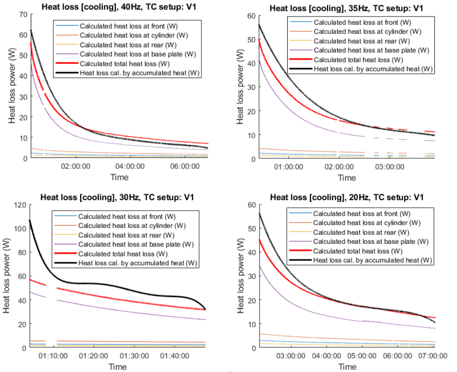
85
equation (3.17), which is based on the temperature measurement and thermal resistance of
heater surfaces. The change in accumulated heat is calculated in three steps. Firstly, the
accumulated heat (kJ) is calculated from the temperature measurement of each component by
equation (3.9). Secondly, the change of accumulated heat (kJ/s) is calculated by average the
change in 5 seconds. Thirdly, a curve to fit the change of accumulated heat was calculated by
MATLAB function ‘polyfit’ with a degree of 6. This step is to filter out the noise from the
temperature measurement.
Figure 3.18: Calculated heat loss in constant frequency tests: (a) 40 Hz, (b) 35 Hz, (c) 30 Hz,
and (d) 20 Hz.
The heat loss in the cooling phase of each test is shown in Figure 3.18. The heat loss calculated
by heat transfer (red line) and heat accumulation (black line) have the similar trend, except the
(a)
(b)
(c)
(d)

86
data of 30 Hz test (bottom left) which has a short length of data that less than an hour and data
interruption for 3 minutes. At the beginning of the cooling phase, the heat loss calculated by
accumulated heat is slightly lower than the heat loss calculated by accumulated heat. This
difference may come from the error of the baseplate temperature measurement because only
the temperature at the centre of the baseplate was measured. As a result, the heat loss to the
baseplate could be underestimated by heat transfer calculation. It is noteworthy that up to 75%
of the heat loss was attributed to the to-baseplate heat loss. It is because the heater has direct
contact with the baseplate without thermal insulation in between (see Figure 3.19).
Figure 3.19: An illustration of heat loss to the baseplate through the front and rear plates. Deep
blue represents low temperature, and yellow and green represents higher temperature. The
temperature at the feet of front and rear plates are lower than other parts of the heater.
Temperature measurement on the core
The temperature of the front and rear of the core was measured by thermocouple TC 3 and TC
10 when the motor was stopped (see Figure 3.12). While the motor is rotating, TC 3 and TC 10
were set at the position that 5 mm away from the core. When the core is stopped, TC 3 and TC
10 were be pushed inward and touched the front and rear surface of the core. Two tests with a
different frequency (30 and 40 Hz) were performed to measure the temperature on the core.
The motor was stopped while the reading of thermocouple TC 2 was at 25, 35, 45 and 55°C.
The temperature profile of the 40 Hz test that stopped at TC 2 reading at 25°C is shown in
Figure 3.20 as an example. Once the motor was stopped, thermocouples TC 3 and TC 10 were
pushed inward and being contacted with the surface of the core, and it took 10–15 seconds for

87
the thermocouples to reach a stable reading. The temperature reading in the transition is plotted
in dot lines. The temperature at the rear surface of the core (TC 3b) is about 3.5°C and 6.6°C
lower than the temperature at the conducting cylinder (TC 2) and the gap filler (based on the
data in Figure A.11 of Appendix A.7), respectively. Notably, this temperature is about 2°C
higher than the temperature of the rear plate (TC 8). This suggests that the heat transfer from
the gap filler to the core through the air gap is more than through the rear plate while HTF is
not introduced into the heater. On the other side, the temperature reading at the front of the
core (TC 10b) has no significant difference with the air gap temperature at the front (TC 10),
and it is about 5°C lower than the temperature reading at conducting cylinder (TC 2). This can
be attributed to the heat loss is high at the front of the heater, which has lower thermal resistance
than the rear of the heater, according to equation (3.17).
Figure 3.20: Temperature profile for the core temperature measurement.
The temperature profiles of the 30 Hz and the 40 Hz test at different stopping temperature were
summarised in Appendix A.9. The results showed the temperature difference between
conducting cylinder and the rear core is about 4°C in 40 Hz test and 3°C in 30 Hz test without
HTF fed into the heaters. These results can be a reference to evaluate the effect of flowing gas
at the air gap as a barrier flow. The temperature difference between the core and the conducting
88
cylinder is expected to be higher because the barrier flow can reduce the heat transfer to the
core through the air gap.
3.5 Discussion
3.5.1 Limitations of wind-driven eddy current heaters for high-temperature heat
generation
In terms of heat generation, an eddy current heater and a resistive heater have the same work
principle, Joule’s first law. However, eddy current heaters can be considered as the combination
of electric generators and resistive heaters. The integration of multiple functions into a single
device may reduce the total costs but causes some technical challenges, especially for the heater
designed for producing high-temperature heat. Two mayor challenges that identified in this
work are discussed as follows.
Firstly, in an eddy current heater, heat is generated on the surface in which only a few
millimetres away to the magnets, and the generated heat can be transferred to the magnets
during the heating process. As a result, the heating temperature of the heater cannot be too high
to maintain the magnets within their working temperatures. Moreover, the heat transfer to
magnets can be a path of heat losses and therefore reduces the efficiency of the heater. Two
methods (i.e. vacuum insulation and thermal barrier flows) discussed in section 3.2.3 can reduce
the heat transfer through the air gap. However, both methods need a sealing system and sealing
components such as labyrinth seals to the air gap and thus increase the complexity of the system.
Secondly, an eddy current heater with typical structure generate heat on a cylindrical surface,
and the fixed shape of heating surfaces limits the design for heat transfer. For comparison, a
resistive heating element can be designed in various shapes which can be surrounded by HTFs.
Further investigation on the above technical challenges is needed to understand how much those
may impact the application of wind-driven eddy current heating technology.
3.5.2 Potential thermal power enhancement
The estimated thermal power of the proof-of-concept heater in the constant frequency test (0.6
kW at 1,150 RPM) is much less than the thermal power that estimated in Table 3.3 (10 kW at
1,132 RPM). The main reason is that the proof-of-concept heater is not aiming for maximising
89
thermal power but building a rig with the flexibility to test different design factors. The thermal
power can be enhanced through the change of the following parameters or designs:
• The number of magnetic poles is 16 in the proof-of-concept heater for the preliminary
tests. According to the data in section 2.2.2, optimising the number of magnetic poles
can increase the thermal power by a factor of two.
• Increase the magnetic field strength through replacing SmCo magnets (1.1 Tesla) by
electromagnets (1.6 Tesla) can potentially double the thermal power based on equation
(3.1) if the other parameters remain the same.
• The total volume of magnets can be increased by changing the shape of the magnets
from the bar shape to the arc shape with the same thickness (6 mm), and this can double
the volume of the magnets on the core.
• Reducing the thickness of the air gap can increase thermal power. A FEM simulation
results [64] shown in Figure 2.7 indicated that the thermal power is increased 30% by
reducing the air gap thickness from 3 mm to 0.5 mm. The air gap thickness of the proof-
of-concept heater is 4.5 mm (7 mm gap with a 2.5 mm of gap filler tube). Thus, there is
still room to reduce the thickness of the air gap. However, this might increase the heat
transfer from the gap filler to the magnets.
Applying the above methods can potentially increase the thermal power of an eddy current
heater by a factor of ten, but those need to be validated by experimental.
3.5.3 Heat loss reduction
The heat loss results in the constant frequency tests (in Figure 3.18) shows that up to 75% of
the heat is lost to the ambient through the heat transfer to the baseplate. Reducing the contact
surface or adding thermal insulation sheets between the front and rear plates to the baseplate
can increase the thermal resistance two times or more. Use low thermal conductivity materials
(e.g. steel and stainless steel, 10–50 W/m.K) to replace the current material (aluminium, 237
W/m.K) can minimise the heat loss as well.
The heat loss to the shaft can be reduced by adding thermal insulation between conducting
cylinder and the front and rear plates. The temperature measurement data shows both the front
and rear plates are being heated up during the heating process, and this heat is then transferred
to the core through the bearing. Adding thermal insulation layers on the front and rear plates to

90
their surfaces contacted the conducting, and outer cylinders could potentially reduce the heat
temperature to the core. Figure 3.21 illustrates the locations of thermal insulation sheets and the
potential temperature distribution change.
Figure 3.21: Illustration of heaters with and without thermal insulation between the front/rear
plates and conducting/outer cylinders. Red, yellow, and blue colour represent high, medium,
and low temperature, respectively.
3.5.4 Design issues and potential solutions
Several design issues were found while assembling and testing the proof-of-concept heater.
Those issues are discussed in the section, and potential solutions are proposed.
Weight and thermal mass of the heater
A heater with a total weight of 45 kg is heavy and difficult to assemble and move the parts of
the heater around by one person. The heat capacity of 23 kJ/K is also too high that it takes 64
minutes to increase the temperature of the heater by 100°C with a 0.6 kW of thermal power.
(a)
(b)

91
High thermal inertia makes it difficult to measure the instant thermal power change. The weight
and thermal mass can be cut down by reducing the size of the heater or using lighter material
for some of the components that do not require high mechanical strength. Replacing stainless
steel by aluminium as the material of conducting cylinder and the outer cylinder can reduce
13% of total weight and 20% of heat capacity.
Figure 3.22: The coupling between the heater and the motor by hubs and coupling torque disk.
Coupling between the heater and the motor
In the preliminary tests, the motor has to be stopped due to the screw on the coupling at the
motor side got loose. Two aluminium hubs are secured to the shafts of the heater and the motor
with two set screws on each hub, and two hubs are coupled by an Oldham style coupling torque
disk (see Figure 3.22). One of the set screws secured on the motor shaft always got loose when
the motor shaft is hot. There is no temperature measurement on the motor and its shaft, but it is
approximately 60–80°C. The set screw will get loose again in a few minutes of running after
retightening the set screw. Several solutions can mitigate this overheat issues. For instance,
changing the type of hubs or the design of the coupling system could reduce the chance of loose
screws. Extra cooling to the motor and running the motor at a lower frequency (e.g. 30 Hz)
could reduce the motor temperature. Using different types of motors (e.g. three-phase motor)
with a suitable power rating that matches to the heater could also reduce the chance of motor
getting overheated.
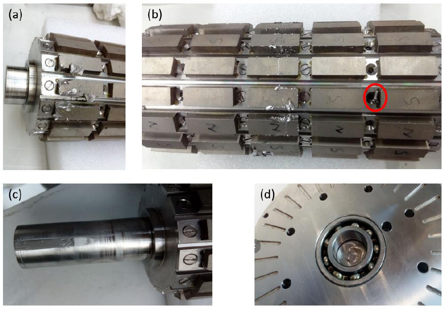
92
Figure 3.23: (a) chipped magnets, (b) a screw got loose on the core, (c) a damaged heater shaft
and (d) failed rear bearing
Parts damage
SmCo magnets are fragile and can get damaged while placing the 4 kg core into the conducting
cylinder with only 5–7 mm gaps (see Figure 3.23a). Once the magnets are chipped or cracked,
it is difficult to remove the small broken fragments from the magnets because those fragments
attract to the magnets. Those fragments could be separated from the magnets when the rotor is
running at a high rotational speed and damage bearings when they fly into the gap of bearings
(see Figure 3.23d).
The screws to fasten the magnet strips on the core could get loose due to the vibration from the
rotating motor and heater (see Figure 3.23b). All of the screws need to be secured and checked
occasionally. If the set screws to hold the hub on the heater shaft got loose, it can damage the
shaft and causes the hub stuck on the shaft (see Figure 3.23c). The set screws on the couplings
need to be fastened correctly.
93
3.5.5 Next steps for investigating wind-driven eddy current heaters
The proof-of-concept heater and models developed in this work can be a good starting point to
investigate and to optimise eddy current heaters for generating high-temperature heat. An
important step is to finish the tests for investigating the correlations of key design factors of the
proof-of-concept heater. Setting up the experimental with a torque transducer and introducing
HTF to the heater (as shown in Figure 3.8) are two important steps to obtain more data from
the proof-of-concept heater. Once the correlation of key design factors is investigated, a FEM
model or mathematical equations can be obtained, like the studies summarised in section 2.2.1.
The results can be used to estimate the device performance such as thermal power and size of
eddy current heaters under different conditions (e.g. rotational speeds). Then a prototype of
wind-driven eddy current heaters can be built to validate the finding in the previous stage. The
proposed next steps for developing wind-driven eddy current heaters are:
The proof-of-concept heater:
• Continue the investigation on key design parameter by set up the heater with full
capability shown in Figure 3.8.
A prototype heater:
• Use the data from the proof-of-concept heater to design and built a prototype heater that
has a higher thermal power.
• Investigate the performance of prototype heater under dynamic operational conditions
(e.g. starting, sudden wind speed change) to simulate real operational conditions.
• Integrate the heater with a thermal energy storage system and study the overall system
performance.
A demonstrator:
• Build and test a heater at a pilot scale, and integrate the heater with a wind turbine.
• Forecast the performance and cost for a large-scale system based on the data from the
demonstrator.
94
3.6 Summary
In this chapter, a proof-of-concept eddy current heater was designed and built to produce high-
temperature heat. This device can be used to investigate the effect of key design parameters and
to estimate the potential performance of eddy current heaters. Unlike existing experimental
studies on eddy current heaters for water heating, this heater is designed to operate under high
temperatures. The magnets installed in the heater can operate at high-temperature (i.e. 200°C).
Compressed air is selected as the HTF, which can operate over 800°C. This heater also has a
design feature (thermal barrier flows) to reduce the heat transfer through the air gap.
Heat transfer and generation models were built to evaluate the thermal power and heat loss of
the heater. A series of preliminary tests were performed to test the mechanical function and the
heating capability of the heater. The results showed that the heater has estimated thermal power
of 620 W at 1,150 RPM, and the heat loss is 50–60 W when the heater temperature is at 40–
50°C. The temperatures of the core in the heater were measured by stopping the motor during
the heating tests. The potential solutions to enhance the thermal power and reduce the heat loss
were discussed. Several design issues that were found in the preliminary tests and their potential
solutions were also discussed. The estimation and demonstration of wind-driven heating
technology is the key to evaluate the cost and system benefits of a direct wind-to-heat system
by comparing it with other systems that can provide the same services, such as a system
integrates electricity-generating wind turbines and electric heaters.
95
4 ECONOMIC ASSESSMENT OF DIRECT WIND-TO-HEAT
SYSTEM FOR ELECTRICITY GENERATION
4.1 Introduction
WTES was first proposed by Okazaki et al. [56] as a system to smooth the electricity generation
of wind power plants by storing wind energy into heat storage and converting heat to electricity.
The preliminary cost analysis in [56] showed that compared to a system that integrates electrical
energy storage, WTES has lower energy costs when large storage capacity (over 24 hours of
storage duration) is needed, due to the low cost of heat storage (see section 2.1.2 for detail).
However, the suitable storage capacity for WTES has not been investigated with wind profiles
being considered, and the cost of WTES has not been compared with systems that store wind
power in heat storage via electrical heating [145].
This chapter aims to understand the potential role of WTES in an electric power system by
investigating the energy costs and appropriate system parameters for different services. An
energy-balance model is developed to simulate the operation of systems that integrate wind
power with energy storage. The LCOE of each system is calculated for different operational
scenarios based on the cost parameters of each component and the energy generation from the
simulation results. The sensitivities of key costs and efficiency parameters are analysed. The
method developed in this chapter addresses the following questions:
1. How should the LCOE of an electricity generation system powered by variable energy
sources and integrated with energy storage be estimated?
2. What are the operational conditions and system configurations under which WTES is
superior to other systems?
4.2 The challenge of high wind penetration in energy systems
Estimating the imbalance between electricity demand and VRE generation allows assessment
of the required power of flexible generation and the curtailed VRE generation. The mismatch
between electricity demand and VRE generation can be represented in a residual load duration
curve (RLDC), which has been used to analyse the need for flexible generation with given
demand and generation profiles [232]. The residual load is defined as the electricity demand

96
minus the generation from non-dispatchable generation sources (e.g. wind, solar, and nuclear),
and it represents the amount of flexible power that is required to balance the electrical grid. The
RLDC presents the sorted residual loads in descending order, usually for a period of one year.
Figure 4.1: A load duration curve against a residual load duration curve [233].
Figure 4.1 shows the load duration curve (on the left) and RLDC (on the right) with four load
bands [233], i.e. peak-load band (first 700 hours ), higher mid-load band (first 2200 hours),
lower mid-load band (first 4400 hours) and base-load band. The share of VRE in an electrical
energy system affects the RLDC and the curtailment of VRE generation. RLDC shifts
downward as VRE share increased, and the load of each band is reduced. When the VRE
generation is over the demand, a negative residual load or curtailment is occurred.
To understand how VRE share affects load bands and curtailment, the UK’s electricity demand
and generation in 2018 [29] are used to calculate the residual load for the analysis. Figure 4.2
shows the RLDC with different VRE penetrations (i.e. 20%, 40%, 60% and 80%; assuming the
ratio of wind generation to solar generation is four) and 16% of base load (representing 6.1 GW
of nuclear power in 2018). As a result, the level of curtailment increases with the share of VRE
exponentially; the curtailment rises from 1% to 21% as the VRE share increases from 40% to
80%. Curtailment is more likely to occur in the transitional seasons between winter and
summer, which have lower electricity demand than winter but relatively high wind and solar
generation. It is notable that the peak residual load mostly occurs in winter, and is only slightly
reduced from 52.3 GW to 50.6 GW with the increase of VRE share from 20% to 80%. This is
because both wind and solar generation are low at residual load peak hours, which most

97
commonly occur during low-wind nights in winter; therefore, the residual load is not greatly
reduced even though the VRE capacity is increased 4-fold.
Figure 4.2: Residual load duration curves with different VRE shares, based on 2018 electricity
data for the UK [29]; seasons are shown in different colours.
Wind generation at different levels of the residual load is affected by the penetration of VRE,
especially when the VRE share is high. Figure 4.3 shows the fraction of wind power generation
in different residual load bands for VRE shares from 10% to 100%. With a 10% VRE share,
the wind generation is evenly distributed in each residual band except the higher mid-load,
which may be because both wind generation and demand are higher in winter. As the VRE
share grows, the fractions of wind generation in the peak-load band and the higher mid-load
band decrease, and the fractions in the base-load band and curtailment band increase. This is
because the wind generation varies significantly with time, such that the generation during high
wind periods can be 5–10 times higher than during low wind periods (see Figure 1.2).

98
Therefore, increasing wind penetration may increase wind curtailment during high wind periods
and only slightly reduce residual load during low wind periods. As a result, the importance of
avoiding VRE curtailment rises significantly when VRE penetration is over 40%. According to
the UK’s net-zero scenarios in Figure 1.1, the VRE share may be 70–80% in 2050, and therefore
55–70% of wind power could be generated during the oversupply time.
Figure 4.3: Wind generation in different residual load bands.
Note that the above analysis is based on electricity demand and generation profiles for 2018.
The demand variations in a single day and different seasons are expected to be larger as a result
of the electrification of the heating and transportation sectors. Using a projected electricity
demand and generation profiles based on future energy scenarios is necessary to produce a more
realistic estimation of the residual load in the future energy mix.
4.3 Methodology for economic assessment
A systematic framework (see Figure 4.4) was built to simulate the operation and estimate the
cost of a power generation system that has input from VRE sources and integrates with energy
storage. The operation of this system is simulated based on energy-balance equations that
consider VRE profiles, operational strategies, and system configurations. The results from the
operational simulation model can be presented in various system operational profiles. The
LCOE of a system can be calculated by a cost estimation model. The NPV of total costs is

99
calculated based on system configuration and cost parameters, and the NPV of energy
generation is obtained from system operation profiles. The results can be used to study suitable
system configurations for different operational strategies.
Figure 4.4: Simulation of variable renewable energy with energy storage.
4.3.1 System configurations and parameters
In this chapter, WTES is compared with two benchmark systems that integrate wind power with
electrical energy storage (EES) or TES. Lithium-ion batteries are by far the fastest growing
EES technology. Their cost has decreased dramatically in the past few years and is expected to
reach 100 $/kWh by 2030 [234]. A 100 MW / 120 MWh lithium-ion battery system was
installed to stabilise the electric grid in South Australia in 2017 [235]. TES is another energy
storage technology that has been deployed for years. Most of the existing large-scale TES
systems are molten salt storage systems integrated with CSP. The cost of TES is much lower
than most electrical energy storage technologies and is targeted to reach 15 $/kWh
th
by 2025
[236]. Different types of TES technologies have been developed and commercialised. A 30
MW / 130 MWh Electric Thermal Energy Storage system using packed-bed rocks as storage
material was built and commissioned in Germany in 2019 [145].
100
Five systems that are configured with different types of wind turbines and energy storage
technology have been selected for analysis (see Figure 4.5). Systems 1 and 2 represent systems
that have electricity-generating wind turbines (eWT) integrated with EES and TES,
respectively. System 3 is a WTES that has heat-generating wind turbines (hWT) integrated with
TES. Note that systems 1 and 2 are classified as non-GIES systems, while system 3 is a GIES
system (see section 1.2.2 for more details about GIES). Compared to non-GIES systems, GIES
systems have more energy conversion steps to produce electricity but have fewer energy
conversion steps to store energy in the storage system. Systems 4 and 5 are hybrid systems that
have both hWT and eWT integrated with TES. Those two systems are included in this study to
investigate the integration of GIES and non-GIES systems. The configuration of each system
is explained below.
System 1 consists of an eWT and EES. An energy converter transforms electricity into another
energy form (e.g. electrochemical) that can be stored in EES. System 2 consists of an eWT and
TES. The electricity generated from the eWT is converted to heat through an electricity-to-heat
(E2H) component (e.g. electrical resistance heating), and the heat is stored in the TES. The
stored heat is converted back to electricity via heat-to-electricity (H2E) components (e.g. steam
turbines and electric generators). System 3 consists of an hWT and TES. Wind power is
converted to heat by the heat generator in the hWT, and the generated heat can be stored in the
TES. Heat is converted to electricity through an H2E component. System 4 is a hybrid system
that consists of both eWT and hWT integrated with TES. In this system, the electricity
generated from eWT can only directly supply to the grid. The heat generated from hWT can be
charged into thermal energy storage, and the stored heat is converted to electricity upon
requirement.
is used to represent the fraction of hWT capacity over total wind turbine
capacity in a system. For example, a 100 MW wind farm with 0.2
has 20 MW of hWT
and 80 MW of eWT. System 5 is a hybrid system that consists of the components of system 4
and an electricity-to-heat component, which allows the power from the eWT to be stored into
TES. Noted that the wind power from hWT is firstly considered to be charged into TES if wind
power needs to be stored, and the power from eWT is considered to be stored only when there
is still excess wind power.
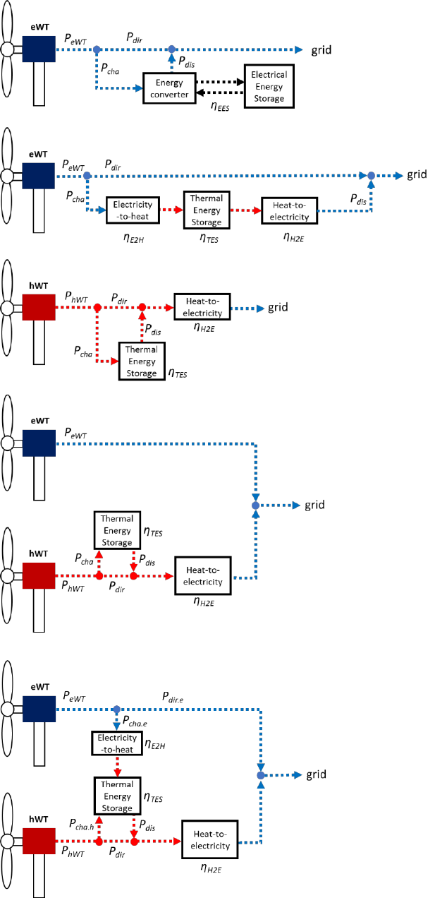
101
Figure 4.5: System configurations of five wind power systems integrated with electrical energy
storage or thermal energy storage.
(a) System 1
eWT + EES
(b) System 2
eWT + TES
(c) System 3
hWT + TES
(WTES)
(d) System 4
eWT/hWT + TES
(e) System 5
eWT/hWT + TES
with E2H

102
The efficiency of each component could be affected by many factors, such as operational
conditions, component lifetime, and the design of the components. For the sake of simplicity,
the efficiency of each component is assumed to be fixed. Table 4.1 summarises the efficiency
of the energy storage and energy conversion components that have been used for analysis in
this work. Since the efficiency may affect the results of the analysis, the sensitivity of key
efficiency parameters (i.e. heat-to-electricity efficiency) is investigated in the section of
sensitivity analysis 4.4.4. Note that the efficiency of a wind turbine for converting wind power
to kinetic energy is not considered in this work, because the focus of this chapter is comparing
the cost and efficiency of different systems. The efficiencies of eWT and of hWT are assumed
to be equal because there is not enough information published about the efficiency of hWT to
better quantify it.
Table 4.1: Efficiency parameters of energy storage and secondary energy converters that
used in the analysis in this chapter.
Symbol
Efficiency
Note
86%
AC-AC round-trip efficiency of lithium-ion batteries [237]
95%
Round-trip efficiency of thermal energy storage
99%
Efficiency of electric heating [238]
41.6%
Efficiency of steam turbines and electrical generators [239]
4.3.2 Cost parameters and assumptions
The costs of different systems are investigated and compared via LCOE analysis. The cost
parameters of most components mentioned in the previous section can be found in literatures,
except for hWT, which is still in the early stage of development. However, the cost of hWT is
expected to be slightly lower than that of eWT due to the following reasons:
• In an hWT, heat generators can replace the components in an eWT that account for 25%
of the capital cost, i.e. electric generators (3.4%), gearboxes (12.9%), power converters
(5.0%), and transformers (3.6%) [120].
• An electromagnetic induction heater can potentially weigh one-tenth of the weight of a
direct-drive electrical generator [56], and will therefore use less material.

103
• hWT requires an HTF circulating system to transfer the generated heat to heat storage
or electricity generation units, but the cost of this system is unlikely to be as high as that
of a generator.
In order to estimate the cost of the system integrated with hWT, the capital cost of hWT is
assumed to be 10% less than that of eWT, and is explored with a sensitivity analysis (section
4.4.4) with an upper bound (same as eWT) and lower bound (20% less than eWT).
Since the costs of wind power and energy storage are falling rapidly, the cost parameters based
on the projection for 2025 (see Table 4.2) are used for analysis in this work.
Table 4.2: Cost parameters of components based on the projection for 2025.
Comp.
Capital cost
O&M cost
Lifetime
(years)
Reference
eWT
1,310 (£/kW)
22,400 (£/MW/year); 5 (£/MWh)
24
[113]
hWT
1,179 (£/kW
th
)
22,400 (£/MW/year); 5 (£/MWh)
24
-
EES
117 (£/kWh)
1.8 (£/kWh/year)
20
[197]
TES
16 (£/kWh
th
)
0.3 (£/kWh/year)
30
[239], [240]
H2E
825 (£/kW
e
)
27,000 (£/MW
e
/year); 1.1 (£/MWh
e
)
30
[241]
E2H
200 (£/kW)
3,000 (£/MW/year)
10
[238], [242], [243]
The assumptions for LCOE analysis are summarised here:
• Electricity-generating wind turbine: the parameters of a >5 MW onshore wind turbine
(61 £/MWh of LCOE) in 2025 are used [113].
• Heat-generating wind turbine: the capital cost of hWT is 10% less than the cost of eWT
in 2025 [113], and the O&M cost is the same as for eWT.
• Electrical energy storage: the cost in 2025 is calculated by the average capital cost in
2019 (312 $/kWh) with a compound annual growth rate (CAGR) of –10% [197]. The
capital cost of EES includes the costs of inverters, storage modules, and balance-of-
system. The ratio of storage capacity to power capacity is 4 hours. O&M is 1.5% of the
capital cost.
104
• Thermal energy storage: the cost in 2025 is projected by interpolating between 25
€/kWh in 2017 [240] and 15 $/kWh in 2030 [239], and assuming that O&M cost is 1.5%
of the capital cost.
• Heat-to-electricity: the projection cost for CSP in [241] is used.
An H2E component
includes steam generation (e.g. steam boilers and pumps, 250 $/kW) and power block
(e.g. steam turbines, condensers, and cooling systems, 835 $/kW). The fixed O&M cost
is 35 $/kW
e
, and the variable O&M cost is 1.5 $/MWh
e
.
• Electricity-to-heat: The estimated cost and lifetime of electric boilers are 60 €/kW and
20 years [238], but those are not designed to charge high-temperature TES. The cost of
high-temperature heaters is discussed in [242], which suggested that the costs of
resistance heaters and associated switches are as inexpensive as a few dollars per kW,
and in [243], which stated that the cost for high-temperature resistive heaters could be
up to 500 $/kW (405 £/kW) based on an interview with a supplier. In this work, it is
assumed that the capital cost is 200 £/kW; a sensitivity analysis uses bounds of 100
£/kW and 400 £/kW. The lifetime is assumed to be half that of the electric boiler due to
operating at high temperature. O&M cost is assumed to be 1.5% of the capital cost.
• Currency exchange rate: 1 USD = 0.81 GBP; 1 EUR = 0.90 GBP.
4.3.3 Operational simulation and cost estimation models
For a wind power system integrated with energy storage, the input power to the system is
determined by wind power profiles, and the output power can be adjusted by storing input
power in storage and discharging it later. In this work, an energy balance-based model was built
to simulate the operation of this system. The UK onshore wind profile in 2016 with one-hour
resolution (see Figure 4.6) was used as the input power profile [22], [23]. The system output is
determined by decision-making algorithms developed to simulate different operational
strategies. System parameters (e.g. power and storage capacities) and component efficiencies
are used as the factors and constraints in the energy balance calculation.

105
Figure 4.6: The UK’s wind capacity data in 2016.
Figure 4.7: Schematic of wind power systems includes all components.
The energy balance equations are based on an all-component configuration (see Figure 4.7)
which includes all conversion and storage components. In this model, the energy conversion in
wind turbines (i.e. from wind power to electricity or heat) is not included. The input power to
the system (
) comes from eWT (
) and/or hWT (
). The power from eWT can be
used to charge the TES (
) or EES (
), or to supply electricity to the grid directly
(
). The power from hWT can be used to charge the TES (
), or to generate
electricity via heat-to-electricity components and directly supply electricity to the grid
(
). The energy balance equations of wind turbine input power are given by

106
(4.1)
(4.2)
The amount of stored energy in EES and TES at time are represented by
and
,
respectively. The energy balance equations of energy storage components are given by
(4.3)
(4.4)
where
and
represent the discharging power of EES and TES, and represents
the length of time for each data point (i.e. one hour in this study). The system output equal to
the input power that supplies electricity to the grid directly and discharging power from energy
storage. The energy balance equation of system output (
) at any time is given by
(4.5)
The constraints of storage capacity and charging and discharging power of energy conversion
components are shown in equations (4.6)–(4.11):
(4.6)
(4.7)
(4.8)
(4.9)
(4.10)
(4.11)

107
where
and
are the maximum storage capacity of EES and TES,
and
are the maximum power of E2H and H2E components, and
and
are the maximum charging and discharging power of EES.
LCOE calculation
LCOE of an electricity generation system can be calculated by NPV of total costs divided by
NPV of total generation. Different methods to calculate LCOE are discussed in section 2.5.1.
In this chapter, the system’s NPV of total cost is calculated by the summation of each
component’s NPV of total cost, and it is given by
(4.12)
where is the total component number,
is the capital cost of component , is the project
year,
is the operational cost of component , and is the discount rate. The lifetime
energy generation is equal to the summation of the system output over the lifetime, and the
NPV of energy generation of a system is given by
(4.13)
where the system output (
) obtained from operational simulation model is assumed not to
change with age. The LCOE of each component can be calculated by the NPV of component
cost divided by the NPV of energy generation. This can be used to analyse the cost of each
component in a system.
4.3.4 Operational scenarios
An energy storage system that integrates with wind farms can be installed at different levels of
electricity networks, i.e. generation side, grid operation, and demand side [48]. This study
focuses on the operation on the generation side since WTES has energy storage integrated at
the generation site. The energy storage system integrated with wind farms can provide several
services, such as time-shifting (e.g. shifting the output from off-peak hours to peak hours),

108
output smoothing (e.g. reducing frequency and voltage fluctuations), and improving
transmission utilisation efficiency (e.g. mitigating transmission congestion) [48].
Three operational scenarios are considered in this study:
• Base load: maintaining constant output to maximise the utilisation of transmission lines.
• Peaking power: shifting all the generation in off-peak hours to peak hours.
• Output firming: reducing the output variation within the forecast horizon and improving the
utilisation of transmission lines without curtailment.
In addition, these scenarios allow us to understand the impact of operational strategies on
system parameters and costs. Unlike in studies that simulate the operation of energy storage
systems by optimising their cost or revenue, decision-making algorithms are used in this work
to simulate the operation of energy storage systems based on the input power and the
operational strategy. Electricity prices are not considered in the model because the price is
affected by many factors and it is difficult to forecast the hourly price in the future. Simulating
the operation with historical price data may underestimate the value of energy storage since the
price variation is expected to be higher in the future. In the end, the results from this framework
can help to understand the system costs, energy flows (e.g. the ratio of energy passing through
storage) and system capacities (e.g. charging/discharging power) for different operational
strategies.
Base load
The base load scenario aims to have a constant system output. An example of a 100 MW wind
power system with an output target of 21 MW is shown in Figure 4.8. The wind power
exceeding the output target is charged to the storage. When wind power is lower than the output
target, the stored energy is discharged to meet the target. In the case that the stored energy is
insufficient to meet the output target, the difference between the target and actual output is
considered as output shortage which can be calculated by equation (4.14). Excess wind power
is considered as power rejection if it cannot be stored in the storage. The percentage of rejection
can be calculated by equation (4.15).
(4.14)

109
(4.15)
Figure 4.8: Example of base load in a one-week operation, during January 17–23, 2016.
Figure 4.9: Base load with different system output targets.
In a system whose charging and discharging power are not limited by the power capacity of the
system, the shortage rate and rejection rate are the functions of the system’s output target as
shown in Figure 4.9. As the output target increases, the rejection rate (blue line) falls and the

110
shortage rate (orange line) rises. The shortage rate is zero at low output targets (e.g. 10 MW),
but the rejection rate is high (e.g. 65%). On the other hand, the rejection rate is low with a high
output target (e.g. 40 MW), but the shortage rate is high (e.g. 32%). In this study, a 5% shortage
rate is selected as the criterion for finding an appropriate output target in order to avoid having
high rejection or shortage rates.
Peaking power
The peaking power scenario simulates the operation of shifting all the output power to peak
hours (defined here as 16:00-21:00, five hours in a day). The wind power at off-peak hours is
stored in the storage system, and the stored energy is discharged at peak hours only. It is
assumed that wind power is rejected if it cannot be stored in the storage system. An example of
a one-week output profile during January 21–27, 2016 is shown in Figure 4.10. During the first
four days, the wind power at off-peak hours is all stored and discharged at peak hours. However,
during the last three days, the storage is full (red line for stored energy) a few hours before the
peak time, and as a result, part of the wind power is rejected. By comparison, the scenario of
peaking power has high output power in a short period of time, whilst the scenario of base load
has low output power evenly distributed over time, demonstrating that the operation strategy
affects the required system parameters.
Figure 4.10: One-week system output profile for peaking power, during January 21–27, 2016.

111
Figure 4.11: One-week system operation for output firming, during January 1–7, 2016.
Output firming
The output firming scenario represents the operation of reducing output variation of wind
generation systems without curtailment. Wind speed sometimes can fluctuate considerably in a
couple of hours, and this operation smooths the system output by storing wind power during
high-wind periods and discharging stored energy during low-wind periods. The system output
target (
) is determined by an algorithm that maximises the utilisation of storage within a
wind power forecast horizon. The algorithm is described in Appendix B.1. Different methods
have been developed to forecast wind power from a few minutes to days ahead [244]. In this
study, a 48-hour wind forecast horizon (
) with no prediction error is assumed. Figure 4.11
shows a one-week example of the operation using output firming. The system output (black
line) is smoothed by storing wind power during high wind periods (purple bars) and discharging
stored energy during low wind periods (yellow bars). It is notable that the stored energy reaches
the storage capacity at the end of the high wind period (e.g. 70
th
and 110
th
hour) and it drops to
zero at the end of the low wind period (e.g. 140
th
hour).
4.4 Results
For the sake of illustration, all results are presented based on a 100 MW wind power system,
using the capacity factor for 2016 as in Figure 4.6. The data are either independent of system
capacity (e.g. LCOE) or can be scaled by the system capacity (e.g. charging and discharging
power capacity). In this chapter, the system’s storage capacity is presented as storage duration,

112
which is defined as the storage capacity divided by the wind power capacity of the system. For
example, a 4-hour storage system has 400 MWh of storage capacity. Furthermore, the fraction
of wind power passing through storage is presented as a charge percentage, which is defined as
the fraction of charging energy over the generated energy from wind turbines and is given by
(4.16)
4.4.1 Base load
Figure 4.12 demonstrates the output profiles of system 2 (eWT+TES) that runs base load
operation for a year with different storage durations, i.e. 0, 10, and 20 hours. For a system with
no storage shown in Figure 4.12a, the system output is only 12 MW, and 63% of wind power
is rejected to meet the criterion of a 5% shortage rate. In Figure 4.12b, the system output rises
to 19 MW, and the rejection rate is reduced by 35 percentage points to 28% when the storage
duration increases from 0 to 10 hours. Notably, a high fraction of power is rejected in the high-
wind periods (e.g. 7.9% of total wind power is rejected during the 510
th
– 990
th
hours, for 19
consecutive days), and a high shortage percentage occurs at low-wind periods (e.g. 23% of total
power shortage occurs during the 3760
nd
– 3970
th
hours, for 9 consecutive days). In Figure
4.12c, the storage duration is doubled to 20 hours, but the system output only increases from
19 MW to 21 MW. Moreover, the rejection rate is only reduced by 10 percentage points to 18%.
This is because the storage capacity is not enough to supply the power during long low-wind
periods.
Figure 4.13 shows results for key indicators (i.e. component LCOE, charge percentage,
rejection rate, and average output) of each system against storage durations from 0 to 20 hours,
based on 2016 wind data. As the storage duration increases, the charge percentage (red line)
and average output (green line) increase because more wind power can be stored during high-
wind periods and later discharged during low-wind periods. It can also be seen that the LCOE
first falls and then rises with increasing storage duration. LCOE reduces because the marginal
cost of adding storage capacity is less than the marginal benefits (i.e. increase system output)
when storage duration is low. When the storage duration is higher than a tipping point, LCOE
increases as a result of marginal cost higher than marginal benefits. Note that systems 4 and 5

113
can have different
, but only the results with
that give the lowest LCOE are shown
here, i.e. system 4 (
) and system 5 (
).
Figure 4.12: Annual output profiles of system 2 for the base load scenario with storage
durations of (a) no storage, (b) 10 hours and (c) 20 hours.
(a)
(b)
(a)
(c)

114
Figure 4.13: LCOE, charging and rejection rate, and average output of systems 1 to 5 with
storage durations of 0 to 30 hours for the base load scenario.

115
Table 4.3 summarises the key results of each system with the lowest LCOE. System 1 has the
lowest LCOE at a low storage duration (2 hours) due to the high capital cost of EES, and
therefore the rejection rate is high (46%). System 2 has a higher storage duration (18 hours) and
a lower rejection rate (25%); however, its minimal LCOE is slightly higher than that of system
1 because of its high costs in E2H and H2E components, i.e. 11.2 and 10.3 £/MWh,
respectively. System 3 has the lowest rejection rate (15%) but the lowest system efficiency
(33%); therefore, its LCOE is higher than those of other systems. System 4 has a lower storage
duration (12 hours) and a higher rejection rate (39%) than systems 2, 3, and 5 because its charge
percentage (11%) is limited by the constraint that only the power from hWT can be stored.
System 5 has the same storage duration and charge percentage but has a slightly higher LCOE
compared to system 2, because the integration of hWT only slightly reduces the capacity of the
electricity-to-heat component from 60 MW to 52 MW, but reduces the system efficiency by
two percentage points.
Table 4.3: The results of each system with lowest LCOE for the base load operation.
System capacities
Operating statistics
Costs (LCOE)
Sys.
(x
hWT
)
Sto.
dur.
E2H
cap.
H2E
cap.
Avg.
output
Cha.
%
Rej.
rate
Sys.
eff.
Total
eWT
hWT
EES/
TES
E2H
H2E
hr
MW
MW
MW
%
%
%
£/MWh
1
2
-
-
16.0
4
46
53
129.1
110.2
-
18.9
-
-
2
18
60
18
19.5
18
25
64
129.5
90.7
-
17.4
11.2
10.3
3
18
-
11
10.0
15
18
33
207.9
-
161.6
33.7
-
12.6
4 (0.2)
12
-
15
15.7
11
39
52
135.2
89.8
20.7
14.4
-
10.3
5 (0.1)
18
52
18
18.8
18
26
62
132.0
84.7
8.7
18.1
10.2
10.4
In summary, the system for base load operation has either a high rejection rate or long storage
duration to regulate the fluctuating wind power to nearly constant output. The results show that
the systems integrated with TES have lower LCOE than the system integrated with EES when
long storage duration is required. However, the lowest LCOE of system 2 is higher than that of
system 1 due to its high cost for energy conversion components (i.e. electric heaters and steam
turbines with electric generators). The system integrated with hWT has a lower capital cost but
a higher LCOE because of its low energy conversion efficiency.
116
4.4.2 Peaking power
Figure 4.14 illustrates the operation profile of the peaking power scenario during the windiest
week of 2016, with system 1 (eWT+EES) and storage durations of 5, 10, and 15 hours. The
profile (Figure 4.14a) with 5-hour storage duration has a rejection rate of 49% in that week. As
the storage duration increases to 15 hours (see Figure 4.14c), the rejection rate drops
substantially, to 3%.
Peaking power scenarios for systems 1, 2, 3 and 5 with storage durations from 0 to 15 hours are
simulated. System 4 is excluded because it has no energy conversion component to store the
power from eWT. Peaking power operation requires high power capacity in order to discharge
the stored energy in peak hours, and the power capacity can affect the LCOE considerably.
Thus, different H2E capacities are simulated, and only the results with the lowest LCOE are
presented here.
Figure 4.15 shows a trend similar to that found in the results for the base load scenario, in that
each system has the lowest LCOE at a specific storage duration. However, the charge
percentage for peaking power is much higher (e.g. over 70% with 15-hour storage), and the
rejection rate is lower as storage duration increases. This is because the peaking power
operation only stores the wind power in off-peak hours (i.e. 19 hours per day in this study) and
discharges stored energy at peak hours (i.e. 5 hours per day).
Table 4.4 summarises the detailed results of each system with the lowest LCOE for the peaking
power scenario. System 1 has the lowest storage duration (6 hours) among all the systems;
therefore, it has the lowest charge percentage and the highest rejection rate. However, system
1 has the lowest LCOE due to its highest average output and higher system efficiency, which
are attributed to the high round-trip efficiency of EES. Systems 2, 3, and 5 have longer storage
durations (10-12 hours), but their overall system costs are 1.6–2 times higher than those of
system 1 because peaking power operation requires high charging power (85–95 MW for E2H
components) and discharging power (50–70 MW for H2E components), and those components
have high capital costs. As a result, the LCOE of charge and discharge components are 3–4
times higher than those of energy storage. Moreover, those systems have low system
efficiencies (i.e. 36–48%) due to low heat-to-electricity conversion efficiencies, and thus have
much higher LCOE than system 1.

117
Figure 4.14: Output profile of system 1 for peaking power in a high-wind-power week with
different storage durations of (a) 5 hours, (b) 10 hours and (c) 15 hours.
(a)
(b)
(c)

118
Figure 4.15: LCOE, charging and rejection rate and average output of systems 1, 2, 3 and 5
with storage durations of 0 to 15 hours for the peaking power scenario.
Compared to systems in the base load scenario, a system in a peaking power scenario requires
less storage duration but higher discharging power. Therefore, the systems that are integrated
with TES have much higher LCOE due to the high costs of energy conversion components. The
peaking power scenario has a higher charge percentage (68%) than the base load scenario
(18%). As a result, the cost difference between a GIES system (system 3) and a non-GIES
system (system 2) is smaller, since GIES is suitable for an operation with a high charge
percentage. However, the LCOE of system 3 is still 20% higher than that of system 2 due to
low system efficiency.
(a)
(b)
(c)
(d)

119
Table 4.4: The results of each system with lowest LCOE for the peaking power operation.
The average output power is calculated in peak hours only (5 hours in a day).
System capacities
Operating statistics
System costs (LCOE)
Sys.
(
)
Sto.
dur.
E2H
cap.
H2E
cap.
Avg.
output
Cha.
rate
Rej.
rate
Sys.
eff.
Total
eWT
hWT
EES/
TES
E2H
H2E
hr
MW
MW
MW
%
%
%
£/MWh
1
6
-
-
107
61
17
74
119.7
79.0
-
40.6
-
-
2
10
95
50
69
68
11
48
197.6
122.1
-
13.0
24.0
38.4
3
12
-
70
52
68
10
36
243.7
-
150.7
20.9
-
72.1
5 (0.1)
10
85
52
68
68
11
47
201.0
112.7
11.6
13.4
22.1
41.2
4.4.3 Output firming
For the purpose of illustration, one-month output profiles of system 4 (
) with three
storage durations (i.e. 0, 3 and 9 hours) are shown in Figure 4.16. For the system with no storage
(Figure 4.16a), the power from eWT and hWT is supplied directly to the grid. For the system
with 3-hour storage duration (Figure 4.16b), the system output (black line) has less variation
because the system stores power from hWT in TES (orange) and generates electricity from
stored heat (TES discharge in yellow). As storage duration increases to 9 hours (Figure 4.16c),
the difference between maxima and minima of system output (black line) on the 5
th
–17
th
days
are further reduced, e.g. the system output on the 8
th
day increases by 7 MW (from 24.5 MW
to 31.5 MW). However, the system output on the 18
th
–20
th
days only increases by 1.3 MW
(from 6.7 MW to 8.0 MW), and one of the reasons is that the storage is not fully charged earlier
on the 16
th
day because the forecast horizon is only 48 hours.
Figure 4.17 illustrates the impact of storage duration on the distribution of hourly system output
over a whole year. As expected, increasing the storage duration narrows the distribution of the
system output, but the impact is smaller once the storage duration is over a certain level. For
example, the output distribution of a wind farm with no storage can be found in Figure 4.17a
with zero hours of storage duration. The minimum and maximum outputs of a wind farm
without storage are 2.2 MW and 96.9 MW, respectively. As storage duration increases to 6
hours, the minimum and maximum output of system 1 change to 6.4 MW and 76.4 MW,
respectively. The distribution then does not change much with the increase in storage duration.

120
Figure 4.16: One-month (January 2016) output profile of system 4 for output firming with
storage durations of (a) no storage, (b) 3 hours and (c) 9 hours. Note that ‘hWT to TES’ is the
thermal power charging into TES and ‘hWT to grid’ is electric power supplied to the grid.
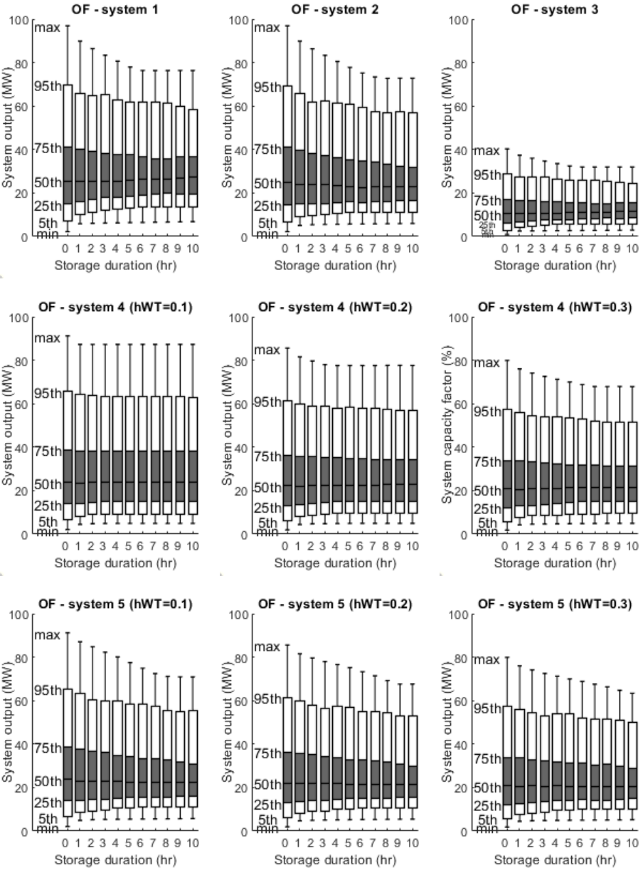
121
Figure 4.17: Box plots of system output at the minimum, 5th, 25th, 50th, 75th, 95th and
maximum percentiles.
(a)
(b)
(c)
(d)
(e)
(f)
(g)
(h)
(i)
122
Moreover, increasing storage duration leads to a reduction in maximum output that is greater
than the increase in minimum input. This is because the charged power is always greater than
the discharged power due to the energy loss in storage. Also, the increase in minimum output
is limited by the length of the forecast horizon, as discussed previously. Notably, each system
shows a different trend in its boxplots. System 3 has the narrowest output distribution due to its
low direct output efficiency. The
parameter affects the boxplot trend in systems 4 and 5:
a low
limits the reduction of the gap between maximum and minimum system output.
The LCOE, charge percentage, and average output of each system with 0–10 hours of storage
duration are shown in Figure 4.18. As the storage duration increases, the LCOE and charge
percentage also increase, while the average output decreases. System 1 has the highest average
system output (green line, 29–30 MW) compared to other systems but its increase in LCOE is
also higher than those of the systems integrated with TES. The LCOE of system 3 (i.e. 170–
180 £/MWh) is much higher than those of other systems, again due to its low direct output
efficiency and therefore low average system output (i.e. 12–13 MW). With the same storage
duration, the LCOE for system 2 is lower than for system 5 but higher than for system 4.
Moreover, the
of system 4 significantly affects its LCOE and charge percentage.
To compare the output distribution of different systems at the same cost basis, a reference cost
of 80 £/MWh is selected because most of the systems have simulation results in Figure 4.18 at
this cost, except system 3. Figure 4.19 shows the impact of the system configuration on the
output distribution at the same LCOE. Notably, system 1 has the highest minimum and 5
th
percentile outputs, and system 4 (
) has the lowest maximum and 95
th
percentile
outputs. Comparing the systems integrated with TES (i.e. systems 2, 4 and 5) in Figure 4.19,
system 2 has the highest minimum and 5
th
percentile outputs and also has high maximum and
95
th
percentile outputs. This indicates that hybrid systems (i.e. systems 4 and 5) have lower
outputs during both high-wind and low-wind periods compared to non-GIES systems (i.e.
system 2).

123
Figure 4.18: LCOE, charge percentage and average output power for the output firming
scenario.

124
Figure 4.19: System output boxplots of system 1, 2, 4 (
0.2 and 0.3) and 5 (
0.1 and
0.2) for output firming scenario at a system cost of 80 £/MWh. The boxplot on the left (Ref.) is
a reference system without energy storage.
Figure 4.20 illustrates the energy flow of different types of systems, based on the system
parameters at the reference cost of 80 £/MWh. In each system, about 12–14% of the input power
passes through storage. System 1 has the lowest energy loss (1.6%), and systems 4 and 5 have
a higher loss (11–12%) than system 2 (8.6%). It is worth noting that the charge percentages of
hWT in systems 4 and 5 are 69% and 60%, respectively. This indicates that the integration of
eWT and hWT can increase the charge percentage of hWT. However, the rest of the hWT
generation (31–40%) does not pass through storage, which is considered an inefficient energy
conversion path for a wind power system; therefore, the energy losses of systems 4 and 5 are
higher than that of system 2.
In summary, the output firming scenario simulates the operation of a wind power system to
reduce its output variation by using energy storage. For a wind generation system, a lower peak
output can prevent wind curtailment and transmission congestion, and higher minimum output
can reduce the need for reserve power to meet the demand during low-wind periods. The results
with the same LCOE showed that the system configuration affects the output distribution of
each system; for example, system 1 has the highest minimum output, and system 4 (
) has the lowest peak output.

125
Figure 4.20: Energy flow of systems 1, 2, 4 (
0.2) and 5 (
0.1) at a reference cost of
80 £/MWh for the output firming scenario.
4.4.4 Sensitivity analysis
The sensitivity of LCOE to five cost and efficiency parameters is investigated with upper and
lower bounds (see Table 4.5). The system configurations for base load and peaking power
which give the lowest LCOE are selected as the base cases, and one of the parameters is changed
while holding others constant. The parameters that affect the costs of all systems, such as the
discount rate and the cost of eWT, are not studied because this work aims to understand the
differences between each system. The following parameters are included in this study:
• Energy Storage cost: the projected costs of EES and TES in 2025 are used for the base
case (see Table 4.2). Due to the uncertainty of technology development and cost
reduction in the future, changes of 50% upward or downward are examined.
• Electricity-to-heat cost: due to the lack of information and the variation in data from
limited references (see discussion in section 4.3.2), a 50% upward or downward change
in the costs is examined.
• Heat-to-electricity cost: the projected cost of the steam generation system and power
block is used as a base case (see Table 4.2). Since the heat-to-electricity technology has

126
been developed for decades, a 20% upward or downward change in the costs is
examined.
• Heat-generating wind turbine cost: the assumption that the capital cost of hWT is 10%
less than eWT is used as the base case (see section 4.3.2). An upward change (equal to
eWT; no cost reduction from converting wind turbines to direct heat-generation) or
downward change (20% less than eWT; significant cost reduction) is examined.
• Heat-to-electricity efficiency: this efficiency can be improved by using a Brayton cycle
for power generation. It uses supercritical carbon dioxide as a working fluid and can
potentially improve the H2E efficiency to 53.8% [239]. The efficiencies of the steam
turbine (base case, 41.6%) and Brayton cycle (upper bound, 53.8%), and an efficiency
midway between these (47.7%), are examined.
Table 4.5: Sensitivity analysis parameters.
Parameters
Lower bound
Base case
Upper bound
Energy storage cost
(ES cost)
-50%
EES: 117 £/kWh
e
;
TES: 16 £/kWh
th
+50%
Electricity-to-heat cost
(E2H cost)
-50%
200 £/kW
+50%
Heat-to-electricity cost
(H2E cost)
-20%
825 £/kW
+20%
Heat-generating wind turbine
cost (hWT cost)
20% less than
eWT
10% less than eWT
The same as eWT
Heat-to-electricity efficiency
(H2E efficiency)
-
41.6%
53.8%
Base load
Figure 4.21 (using system parameters in Table 4.3 as the baseline) shows that the energy storage
cost affects the LCOE more than other cost parameters for each system. This is because high
storage duration is needed for the base load scenario. The enhancement of heat-to-electricity
efficiency can reduce the LCOE of system 3 significantly, but its LCOE is still much higher
than those of other systems. It is worth noting that the LCOE of system 5 (
) is
always slightly higher than or no difference to the LCOE of system 2 at any high or low bounds.
This implies that replacing 10% of eWT by hWT has no change or a negative effect on the

127
system cost. Moreover, the cost of system 4 is slightly lower than that of system 2 only if the
electricity-to-heat cost is at the upper bound. The hWT cost has a limited effect on the LCOE
of systems 4 and 5.
Figure 4.21: Sensitivity analysis for the base load scenario.
Peaking power
Figure 4.22 (using the system parameters in Table 4.4 as the baseline) shows that the energy
storage cost affects the LCOE of system 1 significantly but has less effect on the other systems.
For the systems integrated with TES (i.e. systems 2, 3 and 5), the cost of energy conversion
components (i.e. E2H and H2E) affects LCOE more than the energy storage cost because high
charging and discharging power are required for peaking power. It should be noted that the
enhancement of heat-to-electricity efficiency can significantly reduce the LCOE of the systems
integrated with TES. However, the LCOE for these systems is still much higher than for system

128
1. Moreover, the LCOE of system 5 at any low bounds is always slightly higher than that of
system 2, and hWT cost has limited influence on the LCOE.
Figure 4.22: Sensitivity analysis for the peaking power scenario.
LCOE against charge percentage
For a generation system that integrates energy storage, the LCOE increases as more energy
passes through storage, due to the loss of a portion of the energy in storage. In principle, the
LCOE of WTES can be lower than that of a non-GIES system (i.e. system 2) when the charge
percentage is high enough. The LCOE of a WTES and a non-GIES system at differing charge
percentages with different conditions are investigated based on the following assumptions:
• The charge percentage is independent of system parameters.
• A set of reference system parameters (i.e. 100 MW wind turbines with 20-hour storage,
20 MW of H2E, and 100 MW of E2H) is used as the basis.
• Three cost and efficiency parameters are analysed: hWT cost, E2H cost, and H2E
efficiency. ES cost is not discussed because both systems have the same storage duration.

129
Figure 4.23: LCOE of WTES and non-GIES at different charge percentages for sensitivity
analysis, i.e. capital cost of heat-generating wind turbine (hWT), capital cost of electricity-to-
heat component (E2H) and heat-to-electricity efficiency.
Figure 4.23 illustrates the effect of the charge percentage on the LCOE of WTES and non-GIES
systems. The base case LCOE for the WTES system (180 £/MWh) is much higher than for the
non-GIES system (90 £/MWh) when the charge percentage is 0%. However, as the charge
percentage increases to 100%, the LCOE of the WTES system only increases by 10 £/MWh to
190 £/MWh, and the LCOE of the non-GIES system increases by 160 £/MWh to 230 £/MWh.
In the base case (red and blue solid lines), the LCOE of WTES is lower than the non-GIES
LCOE when the charge percentage is over 84%. By changing the hWT cost (red dashed lines)
and E2H cost (blue dashed lines), the LCOE curves shift up or down, and the crossing point
can occur at charge percentages of 73% to 94%. As the H2E efficiency changes to 53.8%, the
LCOE curve of WTES shifts down significantly, and the crossing point changes to the charge
percentage of 74%.

130
4.5 Discussions
4.5.1 Characteristics of WTES for electricity generation
The characteristics of WTES are investigated in this study by comparing its LCOE with other
systems under different operational scenarios. The efficiency and cost parameters of the energy
conversion and storage systems of each system are summarised in Table 4.6. System 1 has high
pass-through-storage efficiency (86%) and a high storage cost (117 £/kWh) and is therefore
suitable for applications requiring high charge percentage and low storage capacity (e.g.
peaking power). System 2 has a low storage cost (16 £/kWh) and high charging and discharging
power costs, and is therefore suitable for applications requiring high storage capacity and lower
charging and discharging power (e.g. base load).
Table 4.6: The component efficiency and capital cost for each system.
System
Direct-
output
efficiency
(%)
Pass-
through-
storage
efficiency
(%)
WT cost
(£/kW)
Storage
cost
(£/kWh)
E2H /
H2E
power
cost
(£/kW)
1 (eWT+EES)
100
86.0
1310
117
-
2 (eWT+TES)
100
39.1
1310
16
200 / 825
3 (hWT+TES)
41.6
39.5
1179
16
0 / 825
4 (eWT/hWT+TES)
41.6-100
39.5
1179-1310
16
0 / 825
5 (eWT/hWT+TES+E2H)
41.6-100
39.1-39.5
1179-1310
16
200 / 825
System 3 is similar to system 2 in that it has a low storage cost and high discharging power
cost. Moreover, it has advantages in its lower wind turbine cost and in not needing energy
conversion for charging TES, but it has low direct-output efficiency. Therefore, in principle,
system 3 is suitable for an application that has a high charge percentage and lower discharging
power. However, the simulation results showed that these two operational conditions do not co-
exist in a single application if the energy storage is directly charged from wind power. This is
because in an operation with a high charge percentage (e.g. peaking power) more time is spent
in charging the storage than discharging the stored energy; as a result, high discharging power
is needed to release the stored energy in a shorter discharging time. On the other hand, an
131
operation with low discharging power (e.g. base load or output firming) has a comparatively
flat output profile; therefore, the charge percentage is low because only a part of the wind power
needs to be stored to smooth the wind profile. This finding emphasises the importance of
considering real input profiles and system operations of a GIES system powered by VRE (e.g.
wind and solar). As the generation profile of VRE cannot be controlled, the VRE profile affects
the fraction of energy passing through storage and the required system capacities.
4.5.2 The integration of GIES and non-GIES systems
Hybrid systems that integrate hWT and eWT are investigated in this work as systems 4 and 5.
The results show that the integration could cause hWT to operate at a higher charge percentage.
For instance, the results of output firming in Figure 4.20 show that the charge percentage of
systems 4 and 5 is about 14%, but most of the charging power comes from hWT, which has a
charge percentage of 60–69%. However, the results show that a hybrid WTES has a higher
LCOE than a non-GIES system (i.e. system 2) under all the scenarios. This can be explained
by the results from sensitivity analyses that a high charge percentage (i.e. 73–94%) is needed
to make the LCOE of WTES lower than that of a non-GIES system if both systems have the
same capacities. Nevertheless, the simulation results show that each system differs significantly
from the others in the charge percentage and suitable system capacities, even in the same
operational scenario. This suggests that an operational simulation is necessary for comparing
GIES and non-GIES systems.
4.5.3 The impact of integrating wind farms with energy storage
The operational simulation in this study also explores the impact of integrating energy storage
on the costs and output of wind farms. Based on the results in this study, a 100 MW wind warm
has outputs range of 2 to 97 MW and LCOE of 58 £/MWh. For a system that integrates with
storage and operates for base load, the maximum system output could reduce to 16–19 MW,
but the LCOE of the system increases by 71–77 £/MWh to 129–135 £/MWh with 26–45% of
curtailment. For comparison, according to the studies reviewed in section 2.5.2, this base load
operation can avoid additional system costs of 25–80 £/MWh for adding VRE generation into
a power system with high VRE penetration, i.e. 15–45 £/MWh for power reserve, 5–15 £/MWh
for capacity credit and 5–20 £/MWh for transmission and networks.
132
Furthermore, the output firming operation can reduce the maximum output to 76–81 MW and
slightly increase the minimum output to 5–6 MW without curtailment, with the systems that
their LCOE are increased by 22 £/MWh to 80 £/MWh. This can potentially save the additional
costs of 15–45 £/MWh for power reserve.
Those costs indicate that the cost of integrating energy storage with wind farms could be
comparable to additional costs of integrating variable generation into a power system. However,
the later costs are highly depended on the VRE penetration in the electrical system and other
factors, such as the distance for transmission systems of wind farms. Therefore, integrating
wind farms with energy storage could be cost effective if the additional system costs are high.
Since the VRE resources in easy access locations will be developed first, the integration of
energy storage at generation sites is more likely to be deployed in the later stage of the transition
to renewable energy.
4.5.4 The challenge of estimate the costs and benefits of energy storage systems
LCOE is an indicator to compare the cost of different energy storage systems but cannot
represent the value of storage in providing system benefits, especially for the storage system
integrated with generation.
Integrating generation systems with energy storage increases the total system costs and reduce
energy production because the energy loss during storage is unavoidable. As a result, the LCOE
of the system rises but can be justified through the mechanism of electricity markets to increase
the revenue of the systems, such as selling electricity at a higher price or provide grid services.
Electricity markets are designed to translate the need for electric power systems to market
signals or energy prices. Then the dispatchable power generation units and manageable loads
can operate accordingly to maximise their revenue and also the system benefits. However,
estimating the revenue of storage systems requires energy market prices as input. Historical
market prices were used to estimate the potential revenue but not able to reflect the future
market, especially a storage system may operate over 20 years.
This study investigates the cost of modifying the output of wind farms by simulating the
operation of storage for different objectives. This can be an alternative method to evaluate the
benefits of various energy storage technologies for the services that not related to market prices,
such as avoiding transmission congestion or curtailment. For instance, the cost of reducing 20%
133
of maximum output without curtailment is 22 £/MWh. A method to convert the characteristics
of storage systems into indices that can represent the system costs and benefits could make the
assessment of energy storage technologies and other solutions less affected by the assumptions
and input data of individual studies.
4.5.5 The limitation and constrain of this work
The results of this work can be affected by changing the input to the simulation models. The
input data can be divided into two groups: the data for specific systems (e.g. costs of electrical
energy storage for system 1) and general data for all systems (e.g. the wind power profile and
the discount rate for LCOE calculation). The effects of changing key parameters for specific
systems are investigated in the sensitivity analysis, but the effect of changing general data is
not explored. In principle, the change of general data should have marginal effect on the
difference between each system. However, the results in this work are based on the parameters
and assumptions summarised in section 4.3.1 and 4.3.2. The change of input data such as wind
generation profiles or cost parameters could affect the simulation results and the therefore
change the conclusions.
4.6 Summary
We found that the LCOE and output profiles of each system vary considerably with the
objective of system operations. By comparison, the systems that integrate with TES have lower
LCOE for the operation requiring long storage duration, and the system that integrates with
EES has lower LCOE for the operation requiring high discharging power. Notably, the LCOE
of WTES (system 3) is much higher than those of the other systems in all scenarios due to its
low direct output efficiency. The hybrid systems that integrate hWT with eWT can make the
hWT operate at a higher charge percentage (i.e. 60–69% for output firming), but their LCOE is
not lower than the non-GIES system LCOE (system 2). The sensitivity of each system’s LCOE
to the key costs and efficiency parameters is investigated. The results show that the LCOE for
hybrid systems could be lower than for the non-GIES system if the cost of the electricity-to-
heat component is at the upper bound. Furthermore, the LCOE of WTES can be lower than that
of the non-GIES system if the charge percentage is very high (over 73–94%).
134
WTES is a GIES system that requires fewer energy conversion steps to store wind power in
heat storage compared to a non-GIES system. It can be a cost-effective alternative to a non-
GIES system (e.g. storing wind power in heat storage via electric heaters) if a large proportion
of wind power needs to be stored in heat storage. In this work, a systematic framework is
developed to simulate the operation of wind power systems integrated with energy storage
under different operational strategies. The LCOE of WTES and other wind-powered energy
storage systems are estimated and compared. The results show that the LCOE of WTES is
higher than those of other systems because the conditions suitable for WTES cannot exist in a
single operation. Hybrid systems that integrate GIES and non-GIES (or hWT and eWT) are
investigated in this work. The results indicate that the synergy of two types of systems could
make hWT operate at a higher charge percentage, but this is not enough to make its LCOE
lower than that of a non-GIES system. The key findings of this chapter are:
1. WTES has lower LCOE for an operation that has a high charge percentage and low
discharging power. However, those two operational conditions cannot exist in a single
operation because the input power of the system cannot be controlled.
2. The charge percentage of WTES needs to be over 73–94% to make its LCOE lower than
those of non-GIES systems with the same system capacities, (i.e. eWT integrated with
TES).
3. A hybrid system that integrates hWT and eWT can make hWT operate at a higher charge
percentage. However, in the scenarios simulated in this work, the charge percentage is
not high enough to make the LCOE of hybrid systems higher than that of a non-GIES
system.
4. The input and output power profiles have a considerable impact on the LCOE of a GIES
system powered by VRE. Therefore, those profiles need to be taken into account while
assessing the economic value of the GIES system.
The framework developed in this work can be used to investigate the value of other GIES
systems powered by VRE sources, such as a wind-driven pumped heat thermal energy storage
system [74]. More information about the cost and technical properties of hWT is necessary to
better estimate and evaluate its cost and value in an electrical system.
135
5 ASSESSMENT OF DIRECT WIND-TO-HEAT SYSTEM
FOR HEATING APPLICATIONS
5.1 Introduction
Wind power can be converted into heat through various energy conversion routes. In principle,
WTES is the most energy efficient system to turn wind power into heat because it has minimal
energy conversion steps. However, directly converting wind power to heat may not be the most
economical way to use wind power because electricity can be used in different applications and
has a higher economic value than heat. Moreover, heat loss to the environment cannot be
avoided, and hence the system has some restrictions, such as not suitable for long-distance
transmission. Therefore, various criteria such as generation and demand profile and
geographical constraints need to be taken into account to identify the suitable system
configuration for using wind power for heating.
The technical and economic feasibility of WTES for space heating was investigated under
different system parameters (see section 2.1.2 for more detail) [57]. The results showed that the
energy cost of WTES could be competitive to other heat sources such as wood chip boilers and
gas boilers. However, the cost estimation is based on the system integrated with storage systems
that can only supply heat in peak heat demand for two to ten consecutively hours. The profiles
of wind power and heat demand are not considered to estimate required storage capacity, and
the calculation is based on the assumption that no energy loss during storage, which may
underestimate the cost of storage.
The aim of this chapter is to understand the opportunities and limitations of WTES as a system
that converts and stores wind power for heating applications. This chapter is divided into three
parts. Firstly, the correlation between wind power and heat demand is investigated based on
real-life profiles. The required storage capacity to decouple the supply and demand is analysed.
Secondly, two energy conversion routes from wind energy to heat demand through WTES are
compared with two benchmark energy conversion routes (i.e. electrical heating and hydrogen
heating). The advantages and disadvantages of each route are analysed in terms of investment
costs, conversion efficiency, and system integration. Thirdly, the energy costs and system
parameters of a WTES for district heating are studied by considering real-life profiles of wind
136
power and heat demand. This energy cost is compared with the cost of other low-carbon heat
sources. The purpose of this work is to address the following questions:
1. How much storage capacity is needed to balance wind generation and heat demand?
2. What is the benefit of using a WTES as a heat source? What are the operational
conditions that are suitable for a WTES?
3. What is the LCOE of a WTES integrated with a seasonal storage system for space
heating? How is the cost compared to other low-carbon heat sources?
5.2 Energy storage for decoupling wind generation and heat demand
5.2.1 Generation and space heat demand profiles
In the UK and most regions in the world, wind power and heat demand are generally both higher
in winter than in summer. The better overlap of supply and demand means that the number of
backup heat sources or storage capacity could be less. However, wind energy and heat demand
have different patterns in different timescales such as daily and weekly. Figure 5.1 and Figure
5.2 shows the UK’s profiles of wind and solar generation and the heat demand for space heating
in a week and a year. Those profiles are normalised by division at each point by the maximum
value of each profile. The heat demand for space heating is highly dependents on the outdoor
temperature and the daily routine of energy users, such as space heating demand has peaks in
the early morning and early evening (see Figure 5.1). Wind generation can vary anytime, and a
low-wind or high-wind period can last several days. The annual profiles in Figure 5.2 show that
heat demand has larger seasonal variation than wind power, and solar power has an inverse
correlation to the heat demand.

137
Figure 5.1: Normalised wind and solar generation and space heating demand in (a) a week
(January 2–8) [29], [245], [246].
Figure 5.2: Normalised wind and solar generation and space heating demand in a year in the
UK, 2019 [29], [245], [246].
5.2.2 Energy storage to decouple generation and heat demand
Mismatches between VRE generation and heat demand are analysed by calculating the
accumulated difference between generation and demand over a year. The assumptions of this
analysis are:
• The UK’s normalised wind and solar generation profiles in 2019 (see Figure 5.2) are
used as generation profiles [29], [245], [246]. Two types of heat demand profiles are

138
considered: the UK’s space heating profile in 2019 (see Figure 5.2) and a baseload
demand profile (constant demand over a year). Heat demand profiles analysed in this
section are composed of both types of profiles with different baseload heating fractions
from 0 to 100% (see Figure 5.3).
• The annual heat demand of 10 GWh is selected to represent the heat demand of 1,000
households or a medium-scale industrial plant in the UK [139]. Generation and demand
profiles are multiplied by a factor to make total annual generation and demand over a
year to be 10 GWh.
Figure 5.3: Heat demand profiles with different baseload heating fractions (0, 25, 50, 75 and
100%), with annual heat demand of 10 GWh. The baseload heating fraction is defined as the
fraction of baseload heating demand over total heat demand, which is the summation of
baseload and space heating demands.
The accumulated difference between generation and demand is calculated from the first day to
the last day of a year. The results can be illustrated by operating storage systems to decouple
wind generation and heat demand in every data point in a year. When the generation is higher
than demand, the excess energy is stored in a storage. On the other hand, if the generation is
less than the demand, the stored energy is discharged to meet the demand. An appropriated
initial stored energy in the calculation is given to avoid negative stored energy in the calculation.
The maximum accumulated difference represents the minimum required storage capacity for
an energy storage system to decouple the supply and demand. The stored energy at the first and

139
last data point is the same, and this indicates the same annual operation profile will be repeated
if generation and demand profiles are not changed.
Figure 5.4 (a) and (b) show the operational profiles for wind power and solar energy for space
heating, respectively. In Figure 5.4a, excess wind power (orange bars) is stored in storage, and
stored energy (red line) increases during warm months (i.e. June to September) and reaches
maximum capacity (2.2 GWh) in October. The stored energy starts to discharge (blue bars)
from October and the stored energy decreases and reaches zero in May. In the profile of solar
energy for space heating only (Figure 5.4b), it is evident that the amount of charge and discharge
energy is higher than the amount in Figure 5.4a, and the maximum storage capacity (54 GWh)
is also higher.
Figure 5.4: The results of (a) the profile of wind power for space heating, (b) the profile of
solar energy for space heating, and (c) the profile of wind power for demand profile with
baseload heating fraction of 0.7, and (d) storage capacity and percentage with different baseload
heating fractions. Based on the UK’s wind, solar, and space heating demand profiles in 2019.
(a)
(d)
(c)
(b)
140
Figure 5.4c summarise the results of minimum storage capacity and storage percentage for
different energy sources and baseload heating fractions. The storage percentage is defined as
the fraction of demand is met by discharging stored energy. For solar energy, storage percentage
decreases as the baseload heating fraction increased, from 53% for space heating to 28% for
baseload heating. For wind power, the storage percentage is 27% for space heating and slightly
reduce to 22% for baseload heating. Moreover, the storage capacity for wind power has
significant reduction from 2.2 GWh of storage capacity for space heating to 1.1 GWh for
baseload heating. Notably, the required storage capacity for wind power has a minimum value
of 0.6 GWh at baseload heating fraction of 0.7. Figure 5.4d shows the profile of that data point.
It can be found that the stored energy has multiple peaks over a year operation. This means the
storage not only provides capacity for seasonal storage but also for balancing supply and
demand in shorter time scales such as days or weeks. That is the reason that this scenario has a
similar storage percentage (20%), but the required storage capacity is much lower than baseload
only.
The results in this section show that wind power has a more positive correlation to heat demand
than the profile of solar energy, based on the UK data in 2019. About 20–27% of wind
generation needs to be stored to meet the heat demand, and the storage capacity is equivalent
to 6–17% of annual heat demand. This means that large-scale and long-term storage systems
are required. The required storage capacity can be reduced by supplying heat for a mixed heat
demand profile. Please note the results could vary when different wind generation and heat
demand profiles are used as the input of the analysis.
5.3 Comparison of energy conversion routes from wind power to heat users
Wind power can be utilised for heating through various energy conversion routes, and WTES
can be an alternative to conventional systems which have more energy conversion steps, such
as wind-to-electricity conversion and electricity-to-heat conversion. To understand that what
conditions such as transmission distance and storage capacity are favourable for WTES, the
parameters of four wind-to-heat conversion routes are analysed and compared in various
aspects, such as investment cost, energy efficiency and grid integration.

141
Figure 5.5: Possible energy conversion routes from wind power to heat users.
Figure 5.5 illustrates the possible energy conversion routes from wind power to supplying heat
to heat users, including the components for energy conversion, storage and transfer. It is
assumed that the heat demand is met by wind power through one of those routes and no other
heating source to back up. Therefore, seasonal storage is needed to decouple the generation and
supply as analysed in section 5.2.2. The components of those routes are summarised in Table
5.1. Those routes are described as follows.
Table 5.1: The components in four wind-to-heat routes.
Components
Electrical
heating
Hydrogen
heating
WTES with
pipelines
WTES with
transport
Wind power
conversion
electric
generator
electric
generator
heat generator
heat generator
Conversion
at generation
substation
electrolyser
-
charging unit
Transmission
electrical cable
hydrogen
pipeline
heat transfer
pipeline
transportation
Storage
TES
Hydrogen
storage
TES
TCS
Conversion
at demand
substation
electric heater
hydrogen boiler
-
discharging unit
142
In the route of electrical heating, the mechanical energy extracted from wind is converted into
electricity via electric generators. Electrical transmission lines transfer the electricity to the heat
user and then convert it into heat by electric heaters. Substations are required to step up or down
the voltage of the electricity if high voltage transmission lines are used. The generated heat can
be stored in a TES unit. A seasonal storage system to decouple the wind generation and the heat
demand is needed. Large-scale sensible heat storage technologies in Table 2.10 are selected as
the TES technology for analysis in this section due to the technology maturity and low storage
costs.
In the route of hydrogen heating, the electricity generated from conventional wind turbines is
used to produces hydrogen via electrolysers. Hydrogen is then transferred to the heat user
through gas pipelines and converts to heat by hydrogen boilers. Hydrogen can be stored in
various types of hydrogen storage systems.
In the route of WTES with pipelines, the mechanical energy extracted from wind power is
converted into heat by a wind-driven heater. The generated heat is then transferred to the heat
users through pipelines and can be stored in a TES unit. Similar to the route of electrical heating,
large-scale sensible heat storage technologies are selected as TES technologies for analysis.
In the route of WTES with transport, the heat generated from wind-driven heaters is stored in
TES materials through a charging unit (e.g. a thermochemical reactor). The TCS materials are
transported to the heat users and convert back to heat via discharging units. An open-loop TCS
system that uses a solid-gas reaction (i.e. calcium hydration) in fluidised bed reactors is selected
as the TCS technology for analysis [165]. Calcium oxide has low material costs and is widely
available around the world. The technology storing heat in this material is relatively mature
than other solid-gas reactions [164]. More technical and economic details of this technology
are summarised in Appendix C.2. Note that TCS systems also can integrate with electrical
heating systems but not discussed in this section because the aim is investigating the potential
of transferring heat through transporting TCS materials.
Low-carbon heating options have different technological characteristics [247], such as
emissions reduction potential and environmental impact, economic costs and benefits,
consumer experience, and energy system impact. This section aims to compare the key cost and
efficiency parameters and system integration benefits of those wind-to-heat conversion routes.
The cost and efficiency parameters of each component such as energy conversion, storage and

143
transfer are reviewed and compared in the following sections. The potential benefits of grid
integration are also analysed.
5.3.1 Investment cost
The cost of a system that uses wind power for heating is affected by many factors, such as the
scale of the system, terrain and distance between wind turbines and heat users, and the
requirement of heat demand. The investment cost of the components in each route is reviewed
and analysed in order to compare the cost in different system parameters, such as transmission
distance, storage capacity, and storage temperature. The results are summarised in Table 5.2.
The LCOE of the WTES with pipelines route is investigated in a case study in section 5.4.
Table 5.2: The cost parameters of the components of each wind-to-heat route.
Components
Electrical heating
Hydrogen
heating
WTES with
pipelines
WTES with
transport
Wind turbine
(£/kW)
940–1690
940–1690
845–1520
(£/kW
th
)
845–1520
(£/kW
th
)
conversion at
generation
(£/kW)
-
270–350
(electrolyser,
2030)
-
540–990 (TCS
reactor, 2030)
Transmission
(m£/km)
4.2–10
(m£/station)
0.18–0.46
1.2–1.7
0.12–0.35
0.03 (per MW)
Storage
(£/kWh)
0.3–1 (sensible
heat storage)
10–23 (vessels);
0.02 (caverns)
0.3–1 (sensible
heat storage)
0.2 (calcium
hydration)
conversion at
demand
(£/kW)
18–228 (water
heating); 405
(high temp.)
32–228
(hydrogen
boiler)
-
540–990 (TCS
reactor, 2030)
Electrical heating
The projected cost of large-scale (> 5 MW) onshore wind turbines to 2025 (940–1690 £/kW
[113]) is selected for comparison because the transmission system of other routes may be
difficult to build at offshore. The new substation base cost for a 230–500 kV substation without
any equipment is 1.3–2.0 m£/station, and the total cost is dependent on the number of
144
subcomponents such as shunt reactor, series capacitor, and transformer [248]. For estimation,
the total cost of a substation is about 4.2–10 m£/station.
The capital cost of electrical transmission lines is depended on the voltage and power. For
instance, the cost of 72.5kV transmission lines (34–510 MW 0.9 power factor) is 0.18–0.46
m£/km; the cost of 230–600 kV transmission lines with 400–3,000 MW is 0.47–1.05 m£/km
[249]. Note that the installation cost with the same length can be 2-times higher on the terrain
that is more difficult to construct, such as forested and mountain [248]. For comparison, the
capital cost of a substation is equivalent to 10–40 km of transmission lines.
The cost of TTES and PitTES in Table 2.10 is used for the analysis. For water heating, the cost
of 1-10 MW electric heaters is about 20–250 €/kW (or 18–228 £/kW) [238]. The cost for high-
temperature resistive heaters can be up to 500 $/kW (or 405 £/kW) from the interview with
supplier [243].
Hydrogen heating
The current cost of electrolysers is high (700–730 £/kW [250]), and only a tiny fraction of
hydrogen is produced by electrolysis. However, this cost is expected to fall to 270–350 £/kW
as the deployed capacity increased [8], [250]. Hydrogen can be transferred under low or high
pressure. Low-pressure pipelines (40 bar) has lower capital cost than high-pressure pipeline
(1,000 bar), but later one can be used for delivering hydrogen to fuelling stations for fuel cell
electric vehicles. The cost of low-pressure hydrogen pipelines is used for analysis; it is about
1.2–1.7 m£/km (50–1100 mm of diameter; rural area) [251].
The cost of pressurised vessels for hydrogen storage is affected by the manufacturing volume,
and the cost of 300 bar hydrogen storage system with 5.6 kg or 187 kWh is about 10–23 £/kWh
[252]. For very large-scale hydrogen storage (e.g. over 1 TWh), the investment cost of a salt
cavern (typically over 100,000 m
3
) for hydrogen storage is about 9 €/m
3
(or £8.2/m
3
) [253].
This cost per volume is approximately equal to the storage cost of 0.02 £/kWh, based on the
maximum and minimum storage pressure of 200 bar (16.4 kg/m
3
) and 70 bar (5.7 kg/m
3
),
respectively. The information about the cost of hydrogen boilers is limited because hydrogen
boilers are not commercially available yet; therefore, the cost of gas boilers (35–250 €/kW or
32–228 £/kW [238]) is used for analysis due
to the similarity of both types of boilers.
145
WETS with transmission
As discussed in section 4.3.2, the capital cost of heat-generating wind turbines is assumed to be
10% less than electricity-generating wind turbines. The total life-cycle cost of a district heat
network has four main components: network construction, energy loss during peak use, the
annual cost to move energy carriers through pipes, and energy loss in the network [254]. Here
only the construction cost is considered as the transmission cost of the route of the WTES with
pipelines, and it is about 0.12–0.35 m£/km, based on the power of 0.2–4,000 MW
th
with 40°C
of temperature difference [254]. The cost parameters of TES for this route are assumed to be
the same as the electrical heating route.
WTES with transport
In this route, the cost of heat-generating wind turbines is also assumed to be 10% less than
electricity-generating wind turbines. To the best of the author’s knowledge, no TCS technology
is commercialised yet, and there is limited information about its cost. The estimated cost of
TCS is 900–3000 €/kW (or 810–2700 £/kW) in 2015 and expected to be reduced to 600–1100
€/kW (or 540–990 £/kW) in 2030 [255].
The storage and transport cost of the TCS system using calcium hydration reaction was
investigated [165]. In this study, the storage materials (i.e. calcium oxide and calcium hydrate)
are stored in commercial shipping containers, which can contain up to 23.3 tons or 8.6 MWh
of storage materials. This container can be transported by land transportation, such as trucks.
The results showed that the cost per storage capacity is about 0.2 £/kWh, and the transport cost
on land is about 0.53 £/km. In order to compare the transport cost with other routes, this cost is
converted to a lifetime transport cost of 0.03 m£/km, based on 30 years lifetime and 1 MW of
transport capacity. Notably, this transport cost (£/km) per MW is proportional to the number of
containers being transported, or the power capacity of the system; however, the cost of other
transmission systems (e.g. electrical cables and pipelines) has a lower cost per power as the
power capacity increased.
5.3.2 Energy efficiency
Each energy conversion, transfer, and storage components in the routes has an energy loss or
energy consumption. A system with lower energy efficiency means that more input energy is

146
needed to meet the same amount of demand. The efficiency of each component is reviewed and
discussed, and the results are summarised in Table 5.3.
Table 5.3: the energy loss in each part of routes.
Components
Electric heating
Hydrogen
heating
WTES with
pipelines
WTES with
transport
Wind turbine
(%)
5–10
5–10
<5
<5
Conversion at
generation (%)
<1 (substation)
18–28
COP >1 (heat
pump)
34 (charge
efficiency); 2
(axillary)
Transmission
(%)
4-15
<1
<20
0.3-0.8 (per 10
km)
Storage (%)
10–40 (TES)
11-13 (HP); 30
(liquid)
10-40 (TES)
<1 (self-
discharge)
Conversion at
demand (%)
<1 (electric
heating); COP >1
(heat pump)
9-15
-
2 (axillary)
Electrical heating
In general, the overall efficiency of the electrical heating route is higher than the route of
hydrogen heating but lower than the route of WTES with pipelines. In electricity-generating
wind turbines, about 5–10% of energy is lost as heat in the conversion from kinetic energy to
electricity [77]. The energy loss in the substation varies with the specification of transformers
and its operational condition, but it is marginal (<1%) compare to the loss in other components
[256], [257]. The energy loss in electrical transmission systems can be affected by technical
(e.g. length of transmission lines, the voltage of the grid) and non-technical factors (e.g. energy
theft), and the technical losses in transmission and distribution grid is about 4–15% [258].
The storage efficiency of a TES system varies with its technology. For the thermal energy stored
in sensible and latent heat, the stored energy is lost by heat transfer to the environment, and it
is proportional to the temperature difference between storage materials and the environment.
For this route, the storage efficiency of TTES and PitTES (see Table 2.10) is used for analysis.
The efficiency to produce heat from electricity is high. Electric heaters have energy conversion
147
efficiency almost 100%, and electric heat pumps can use one unit of electrical energy to produce
2–4 unit of heat [259].
Hydrogen heating
The overall energy efficiency of the hydrogen heating route is lower than other routes due to
high energy loss in producing hydrogen and reducing storage volume. The energy efficiency of
each electrolysis technology is different, such as alkaline electrolysers (62–82%) and proton
exchange membrane electrolysers (67–82%) [260]. The efficiency of those technologies is
expected to reach 82% after 2030 [8], and the projected net system efficiency can reach 72%
[250]. Hydrogen could lose to the environment at different components in transmission
systems. About 0.5% is lost at compressors, and the loss in transmission pipelines is about 486
kg/km in a year, or 2.2 kW/km [261]. This is very low compared to the loss of electrical
transmission lines (about 220 kW/km [165]).
For reducing the volume of hydrogen, compressing hydrogen to 350–700 bar consumes a
significant amount of energy, which is equal to 11–13% of hydrogen’s energy content.
Liquefying hydrogen can further reduce its volume and make it able to store at ambient
pressure, but this consumes more energy which equals to 30% of its energy content [176].
About 15% of hydrogen’s heating value is released in the form of the evaporation heat of the
water. This means 15% of the energy stored in hydrogen will be lost if the evaporation heat of
water is not used in the heating process. For comparison, natural gas has 10% of heating value
in the evaporation heat of water, and gas boilers can recover about 4% of natural gas’ heat value
by condensing water vapour [262]. Based on the data on gas boilers, it is assumed that hydrogen
boilers can recover up to 6% of hydrogen’s heating value.
WTES with pipelines
The energy conversion efficiency in the route of WTES with pipelines is higher than other
routes, but the transmission efficiency is more sensitive to the length of pipelines. There is no
studies or experimental data about the efficiency of heat-generating wind turbines, but the
energy loss is expected to be lower than electricity-generation wind turbines (5–10% [77])
because electrical conversion components are needed. Thus, the loss in heat-generating wind
turbines is estimated to be less than 5% in this analysis. The energy loss in heat networks is
highly depended on the length of transmission lines, the temperature of transfer fluid, and the
148
thermal resistance of thermal insulation layers. In general, the heat loss in a district heat network
is no more than 20% [186]. The efficiency of storage is assumed to be the same as the route of
electrical heating because both routes store heat in TES. No further energy conversion is needed
at the heat users because wind power is converted into heat at the generation already.
WTES with transport
The route of WTES with transport has comparatively high efficiency at each component except
charging units. The storage efficiency of solid-gas thermochemical storage can potentially as
high as 95% if sensible heat is stored in the storage system [164]. However, storing high-
temperature sensible heat requires thermal insulation layers to reduce the heat loss to the
environment, and it is not economical for long-term storage (e.g. weeks to months). Based on
the analysis of open-loop calcium hydration system in [165], the charging efficiency is about
66%, and the rest of the heat is stored in water vapour, which can be used or stored at low-
temperature (<100°C). The study also showed that the energy consumption for land
transportation is about 0.3–0.8% per 10 km of end-to-end distance. This is calculated based on
the assumption that the energy consumption of electric truck is half of the truck with a
combustion engine (4 kWh/km [263]) and a truck can transport 23.3 ton (or 8.6 MWh) of TCS
materials. In the charging and discharging process, additional energy is needed for pumping
and particle transportation, which equals to 4–5% of stored energy [164].
5.3.3 Grid integration
Integrating local energy systems to the region or national grids can benefit the whole energy
system by increasing the flexibility of the system. If two energy system has different generation
and demand profiles, connecting two systems can reduce the peak of overall generation and
demand and reduce the requirement of flexible capacity [264].
In the routes of electrical heating, the transmission system can connect to electrical grids if their
specifications such as voltage and frequency are the same. If not, those parameters can be
adjusted and matched by the transformers in substations. The grid integration allows the local
TES system to provide daily and weekly flexibility to the grid. For example, the excess wind
generation in local systems can export to the grid during peak hours, and the off-peak electricity
from the grid can be stored in the local TES.
149
In the route of hydrogen heating, local hydrogen pipelines can connect to hydrogen networks if
the pipeline pressure is matched. Connecting local hydrogen pipelines to the hydrogen networks
allow local systems to access the storage facility in the hydrogen networks. This can reduce to
cost for storage system because hydrogen storage has a lower cost at scale.
For the route of WTES with pipelines, in principle, the integration to the other heat networks
that have different demand profiles can reduce the required storage capacity for local systems
(see the analysis in section 5.2). However, heat transfer pipeline is unlikely to connect to the
other heat networks due to its high energy loss in long-distance transfer, especially for high-
temperature heat.
The route of WTES with transport delivers energy through transportation systems and therefore
can deliver to different locations without installing pipelines or cables. However, specific
facilities such as discharging systems are needed to convert the stored energy in TCS materials
back to heat. As a result, implementing this TCS system in heat users that have different demand
profiles may reduce the overall storage capacity, but this has little impact on the overall system
cost because the major cost component of TCS systems is the discharging units.
5.3.4 Characteristics of wind-to-heat routes and suitable operational conditions
Each route has its characteristics and therefore is suitable for different operational conditions.
The cost and efficiency parameters collected in previous sections are summarised in a
comparison table (Table 5.4), which is used for the analysis in this section.
The route of electrical heating has moderate costs and energy loss for energy conversion units,
compared to other routes. Electrical transmission systems have high investment cost for
substations, but the transmission line has comparatively low cost and low energy loss.
Therefore, it is cost-effective for long-distance transmission. Large-scale sensible heat storage
has higher energy loss than hydrogen storage and TCS, but it can be used for grid balancing if
the system is connected to the grid. This can increase the economic value and utilisation of the
storage system.
The route of hydrogen heating has high costs and energy loss for energy conversion units.
However, the cost of hydrogen storage at a very large scale is much lower than other storage
technologies, and the storage loss with time is low. As a result, this route is suitable for long-
term storage (e.g. months to years). The cost of hydrogen pipelines is higher than other

150
transmission systems, but connecting to the hydrogen network could bring down the cost of
storage by sharing the storage on the network.
For local heating systems, the route of WTES with pipelines has lower investment cost and
energy loss than other routes. This route has fewer energy conversion steps, and its transmission
cost (e.g. £/km) is low. However, the transmission distance of pipelines is limited due to its
high heat loss to the environment. This also indicates that this route is not able to provide
additional value through grid integration, which usually requires long-distance transmission.
The route of WTES with transport have high investment costs for conversion components (i.e.
TCS reactors) and energy loss for energy conversion, but low transportation and storage costs
at a small scale. Therefore, this route could be more cost-effective for small-scale systems
required low discharging power.
Table 5.4: Summary of the comparison of system flexibility, cost and efficiency of each route;
‘+’ for advantage and ‘-’ disadvantage.
Electrical
heating
Hydrogen
heating
WTES with
pipelines
WTES with
transport
Conversion cost
+
-
++
--
Conversion efficiency
+
--
++
--
Transmission cost
-
--
+
++/-
*
Transmission efficiency
+
++
--
-
Storage cost
+
--/++
**
+
++
Storage efficiency
-
+
-
++
System integration benefit
++
+
--
-
* The transportation cost of WTES with CST is cost-effective for small power.
** The cost of hydrogen storage is high for small scale, but very low at TWh-scale.
In summary, the route of WTES with pipelines has lower investment cost and energy loss and
may be suitable for using wind power for district heating in a local region. The cost and system
parameters for this application are investigated in a case study in section 5.4. However, when
grid connection is geographically and economically feasible, the routes of electrical heating and
hydrogen heating should be considered first because the benefits those can bring to the whole
system. In the end, the route of WTES with transport may be suitable for small scale heating
system, but further technology development and assessment are needed.

151
5.4 Cost analysis of direct wind-to-heat system for district heating
Cao et al. [57] investigated the energy cost of WTES that uses different wind-driven heating
technologies for space heating. This study was aimed to investigate the impact of heating
technologies and system parameters on energy costs. The impact of storage capacity was not
fully explored because only two to ten hours of storage duration is used in the analysis, and this
storage capacity is not enough to balance the supply and demand in different seasons over a
year. As a result, some wind generation may be curtailed in the season while heat demand is
low, and some heat demand cannot be met by the system while wind generation is low and heat
demand is high. The heat loss during storage affects the required storage capacity and has not
investigated yet.
The main objective of this section is to fill the research gap by considering generation and
demand profiles and energy loss during storage. A district heat network for space heating with
10 GWh of annual heat demand, which represents the heat demand of 1,000 households in the
UK [265], is selected as the basis for analysis. The WTES integrates with a large-scale sensible
heat storage system (see Figure 5.6) and is assumed to be the only heat source of this network.
The UK’s domestic gas and wind generation profiles in 2019 with one-day resolution in Figure
5.2 are used as the input for an energy-balance calculation, which is the same method used in
section 5.2. The system parameters such as required wind power capacity and storage capacity
are calculated by considering different storage efficiency.
Figure 5.6: Proposed wind-powered thermal energy system configuration for district heating.
5.4.1 System parameters for cost estimation
The system parameters of WTES with storage efficiency from 50% to 100% (see Table 2.10)
are discussed. Figure 5.7 illustrates the annual operational profile of a WTES with storage

152
efficiency of 70%. The stored energy in the first and last day of the calculation is the same,
which means the generation in a year is enough to meet the demand. Notably, the surplus wind
generation (orange bars) between May to October is stored in heat storage and discharges (blue
bars) in the winter and spring.
The required wind power and storage capacity with different storage efficiency are shown in
Table 5.5. As the storage efficiency decreased, wind power capacity is increased to compensate
for the energy loss during storage. At the same time, the discharge percentage, which is defined
as the fraction of heat demand that meets by discharging heat storage, is falling. This is because
a higher wind power capacity not only increases the excess generation to be stored but also
increase the generation when demand is higher than wind power. The storage capacity of 2.4–
3.1 GWh equivalents to a 29,500–51,100 m
3
of TTES (energy density 60–80 kWh/m
3
) or a
47,100–102,200 m
3
of PitTES (energy density 30–50 kWh/m
3
).
Figure 5.7: The profiles of heat demand and operation of heat storage for district heating with
10 GWh of annual heat demand, based on storage efficiency of 70%.

153
Table 5.5: System parameters for district heating.
Storage efficiency
50%
70%
90%
100%
Wind turbine power capacity (GW)
5.8
5.6
5.3
5.2
*Discharge percentage (%)
20.3
23.2
25.5
26.6
Storage capacity (GWh)
3.1
2.6
2.4
2.2
Extra wind capacity (GW)
0.6 (+12%)
0.4 (+8%)
0.1 (+2%)
baseline
Key assumptions: annual heat demand is 10 GWh; wind power capacity factor is 0.22,
average onshore wind capacity factor in Europe in 2018 [266].
5.4.2 LCOE of WTES integrating seasonal storage
The LCOE of a WTES with seasonal storage is analysed and compared with other low-carbon
heat sources. Firstly, the LCOE of seasonal storage is estimated based on the wind power and
storage parameters obtained in Table 5.5. This LCOE is calculated by NPV of storage cost
divided by NPV of wind power generation. The equation for LCOE is shown in equation (2.17).
Figure 5.8 shows the LCOE of storage with different parameters, such as storage efficiency,
storage costs, and lifetime. It can be observed that the impact of storage capital cost on LCOE
is higher than storage efficiency and lifetime. The lifetime of the storage system has less impact
on the LCOE because the calculation considers discount rate and O&M costs. The LCOE of
seasonal heat storage is in the range of 6–20 £/MWh, without considering the additional 2–12%
of wind power to compensate for the energy loss during storage.
Secondly, the LCOE of a WTES integrated with seasonal storage is estimated based on the
results in [57]. Figure 5.9 shows the LCOE of WTES without seasonal storage (result from Cao
et al. [57]) and with seasonal storage. Two heat generation technologies (i.e. electric boilers and
mechanical heat pumps) represent the technology that has the highest and lowest LCOE.
Notably, the LCOE of the system with electric boilers is about 50% higher than mechanical
heat pumps, and adding seasonal storage to a WTES increases the total LCOE by 17–36%. This
indicates that the cost of seasonal storage affects the LCOE considerably.
For comparison, the LCOE of wood chip boilers is about 66–90 £/MWh [57], and the projected
retail price of hydrogen produced from electrolysis is about 100–130 £/MWh, which is
calculated based on the assumption that the retail price is 2–2.2 higher than market price (50–

154
60 £/MWh after 2040 [267]. This suggests that WTES using mechanical heat pumps and
integrated with seasonal storage has lower LCOE than hydrogen boilers and comparable to
wood chip boilers.
Figure 5.8: Levelised cost of storage of heat storage with 0.3, 0.5 and 0.8 £/kWh of capital
cost, storage efficiency 50, 70 and 90%, and lifetime 20, 30, 40 and 50 years; based on the
discount rate of 7% and O&M costs is 0.7% of the capital cost.
Figure 5.9: LCOE of WTES for district heating with different wind-driven heating
technologies (i.e. electric boilers and mechanical heat pumps) and wind power capacity factor
(0.15–0.3); blue lines present the results from [57] (without seasonal storage); orange lines
present the LCOE with seasonal storage (storage efficiency 70%; capital cost 0.5 £/MWh).

155
Increasing wind turbine capacity to generate more heat can reduce the required storage capacity
but also increase the curtailment. However, this trade-off can reduce energy costs only if the
cost of wind turbines is low and the cost of storage is high. Figure 5.10 shows the correlation
between the increase of wind turbine capacity and the reduction of storage capacity, based on
the wind turbine capacity and storage efficiency in Table 5.5. Figure 5.10a shows that
increasing 5–20% of wind turbine capacity reduces 13–44% of storage capacity. Furthermore,
the system has a higher storage efficiency (i.e. 90%) has a slightly higher reduction of storage
capacity than the systems with lower storage efficiency. This can be attributed to a higher
storage efficiency system has a higher discharge percentage (see Table 5.5), and the ratio of
wind turbine capacity to storage capacity is therefore higher. Figure 5.10b shows the ratio of
storage capacity reduction to the increase of wind power capacity. It can be observed that this
ratio is in the range of 2.2–3.1 and reduces as the increase of wind turbine capacity increased.
This means that the trade-off has cost benefits only if the cost of wind turbines is less than 2.2–
3.1 times of storage cost. Based on the storage cost of 6–20 £/MWh, the cost of wind turbine
needs to be less than 13–62 £/MWh, which is not much lower than the cost in Figure 5.9.
Figure 5.10: The correlation between increasing wind turbine capacity and (a) the reduction of
storage capacity and (b) ratio of storage capacity to wind turbine capacity; with storage
efficiency of 50%, 70% and 90%.
5.5 Discussion
Wind power can be an appropriate energy source for heating in the cold climate regions that
have high wind resources, such as Scotland and northern European countries. Both wind
generation and heat demand are high in winter than summer. Based on the UK’s demand data,
(a)
(b)
156
20–27% of wind generation is mismatched to the space heating demand and need to be stored
and dispatch at another time. For comparison, the mismatch between solar energy and heat
demand is over 50%.
WTES has the potential to be one of the low-carbon heating options for decarbonising heating
sectors. The results in this study show the LCOE can be competitive to other low-carbon heating
solutions, and this system has cost and efficiency advantage in specific circumstances. For
instance, the cost of grid connection is high, and the location of wind resources is not too far
(e.g. < 100 km).
WTES also has many limitations that may affect its development. Firstly, turning wind power
into heat at generation sites increases the difficulty to transfer generated energy in long-distance
and to convert it into another form of energy. Therefore, converting wind power to heat is not
the first choice for using wind energy. Secondly, WTES is a centralised heating system that
needs corresponding facilities to utilise those heat, such as district heating networks and
radiators. Equipment or system upgrades are necessary if the existing heating system is
decentralise heating systems, such as electric heaters and gas boilers.
WTES is a merging technology that further research and development are needed. One of the
crucial parts is developing and demonstrating the wind-driven heating technology that can
operate under varying wind speeds. The heat storage system also needs to have the capability
to charge and discharge with the variation of both wind generation and heat demand. In the end,
a geographical survey can help to identify the potential location for installing this system. For
instance, a place has heat demand and close to wind resources, and the cost for grid connection
or upgrade is high. The large-scale TES integrated with the system can still be used to store off-
peak electricity via electrical heating within the existing transmission capacity.
5.6 Summary
In this chapter, a system that converts wind power into heat in wind turbines and stores in large-
scale storage was studied. Firstly, the storage capacity of a wind-to-heat system to fully
decouple wind generation and heat demand was investigated by considering the annual profiles
of wind power and heat demand. The results show that both profiles have a positive correlation,
but over 20% of wind power needs to be stored to meet the demand in heating seasons. A mixed
157
of space heating and baseload heating demand could reduce the required storage capacity
substantially.
Secondly, different energy conversion routes from wind power to heat demand were reviewed
and compared with WTES. The analysis shows that WTES integrated with heat networks has
low investment cost and low energy loss with short transmission distance (< 100 km). However,
this system lacks the potential for grid connection, which can bring benefits to both the local
system and the grid. The WTES using TCS for storage and transport was also investigated. The
results suggest that this system has a low cost for delivering heat in small scale, but the
economic feasibility is not clear due to its high cost of charging/discharging units.
Thirdly, the LCOE of WTES that integrates with seasonal storage was studied with the
consideration of wind power and heat demand profiles and different storage parameters. The
results indicate that 2.4–3.1 GWh of large-scale sensible heat storage is needed to fully decouple
wind generation from a 10 GWh of annual space heat demand. Integrating seasonal storage
increases the total LCOE by 17–36%, but it is still lower or comparable to other low-carbon
heat sources.
158
6 CONCLUSIONS AND FUTURE WORK
WTES is a novel system which may provide alternative means of harnessing wind power, and
this thesis is the first work to comprehensively review and assess WTES for electricity and heat
generation in the context of technical and economic feasibility. In this work, different wind-to-
heat technologies are carefully reviewed, and eddy current heaters are selected to be further
investigated for high-temperature heat generation. A proof-of-concept eddy current heater was
designed and constructed to test various design parameters. The technical challenges of this
wind-to-heat technology were discussed and analysed. The roles of WTES for electricity and
heat generation were investigated by comparing with other system configurations or routes that
can provide similar services, such as electricity-generating wind turbines with electrical heating
and thermal energy storage. The results and analysis in this work describe the opportunity and
limitation of WTES as an alternative to conventional wind power systems. The methodologies
for the economic assessment can be applied to other generation-integrated energy systems.
6.1 Conclusions
Wind-driven heating technology
Wind-driven heating technologies are the core of a WTES because the system’s advantage is
attributed to its single energy conversion step to produce heat from wind power, compared to
conventional wind power systems that require two conversion steps to produce heat. However,
the potential cost saving and energy loss reduction from the direct wind-to-heat conversion is
marginal. The analysis in this work shows that the potential reduction in capital costs is up to
20% and energy loss reduction is up to 5–10%.
Eddy current heating technology has the potential for producing high-temperature heat at low
rotational speeds with less device weight, compared to direct-drive electric generators. The
technical challenges are how to reduce the heat transfer from the heating surface to magnets
without losing heating power, and how to reduce the heat loss at coupling and mechanical
support components.
A proof-of-concept device was designed and built for high-temperature heat generation. The
device’s capability for the parametric study has been demonstrated, but more experimental
159
works are needed to understand the correlation between key design factors and operational
parameters.
WTES for electricity generation
WTES have minimal energy conversion steps and components to store wind power in heat
storage. However, the process of converting heat into electricity has low efficiency with over
half of energy lost, and the system for heat-to-electricity conversion has high investment costs.
In principle, WTES could have lower costs in applications required both a high fraction of
energy passing through storage and low power capacity for electricity generation. However, the
simulation results show both conditions do not exist in a single operational strategy as the input
power (i.e. wind power) to the system cannot be controlled. The sensitivity analysis estimates
that WTES may have cost advantages when at least over 73% of wind power needs to be stored
in heat storage, compared to systems that integrate electricity-generating wind turbines and
thermal energy storage. The simulation results indicate that the integration of heat-generating
wind turbines and electricity-generating wind turbines may increase the energy passing through
storage for WTES but still less than 70%. A whole energy system simulation is needed to further
explore the potential roles of WTES in electrical energy systems.
WTES for heating applications
The cost and energy loss of WTES for heat generation can be lower than conventional systems
that use electrical heating or hydrogen heating. However, the deployment of WTES has several
limitations and restrictions, such as limited transmission distance (< 100 km) and low feasibility
for other energy uses. Other wind-to-heat routes that convert wind power to an intermedia
energy form such as electricity and hydrogen may have higher investment costs and energy loss
than WTES. However, those intermedia energy forms are able to transfer in long-distance (over
100 km) and can be integrated to other energy systems or non-heating sectors. Therefore, WTES
can be an alternative system for heating and enables the use of wind energy when grid
connection is not feasible or not cost-effective. As a result, the utilisation of wind energy at
some places such as remote area may be improved.
160
6.2 Future work
Wind-driven heating technology
The development of electromagnetic induction for directly convert kinetic energy to heat is still
in the early stage. The investigation of the technical feasibility and limitation of this technology
is the key to evaluate the potential cost and value of WTES. The proof-of-concept device
constructed in this work can be used to study the correlation of key design parameters and
further estimate its device performance. Once the potential of this technology has been explored
and demonstrated, further investigation under real-life operational conditions is needed to
understand the performance under different wind conditions.
WTES for electricity generation
The suitable application of WTES in an electric power system is still unclear. A whole energy
system modelling that includes WTES and alternative systems can help to understand the role
of WTES in the future energy system. Since the VRE penetration affects the need for energy
storage, the future energy mix and electricity prices should be considered in the economic
assessment.
WTES for heating
The cost and system parameters of WTES for heating are highly depended on the geographic
conditions and the profiles of wind power and heat demand. A survey of the location of existing
heat users, potential wind turbine installation, and electrical and hydrogen grid can show the
potential of this system. Case studies with real-life data (e.g. geographical information, heat
demand, and wind generation) are needed to evaluate and compare the energy cost of WTES
and other routes.

161
A. APPENDIX: WIND-DRIVEN HEATING
TECHNOLOGY
A.1 Radiation heat transfer at the air gap
Figure A.1: Radiation heat transfer between two long concentric cylinders [268].
The radiation heat transfer between two plates (see Figure A.1) can be written as:
(A.1)
where is the heat transfer rate (), is the Stefan-Boltzmann constant (
),
and
are the area of the radiation surface of two long concentric cylinders (
),
and
are the temperature of cylinders (),
and
are the emissivity of cylinders. At the
air gap, the radiation heat transfers from the inner surface of conducting cylinder or the gap
filler to the core. In the proof-of-concept heater, the surface on the core is not like a smooth
tube since the bar-shape magnets and metal strips are attached on it, and, therefore, it is difficult
to estimate the effective surface area for the radiation heat transfer on the core. To evaluate the
radiation heat transfer at the air gap, it is assumed that:
• The surface of the core is like a smooth tube shown in Figure A.1.
• The dimensions of the conducting cylinder (i.e. 0.2 m in length and 0.1 m in diameter)
and the core with magnets (i.e. 0.2 m in length and 0.093 m in diameter) are used for
the calculation.

162
• The temperature of the core is always at 20°C (T
2
)
The emissivity of a surface varies with the surface roughness and its material (see Table A.1).
Figure A.2 shows the heat transfer rate at the air gap with different emissivity and temperature.
The results show the radiation heat transfer can be reduced by reducing the emissivity of the
surface. Moreover, the radiation heat transfer at the air gap is relatively low compared with the
designed power of proof-of-concept device (i.e. 10 kW).
Table A.1: The emissivity of common metals and surfaces [269].
Material
Surface
Temperature (K)
Emissivity
Aluminium
Highly polished plate
500-850
0.039-0.057
Polished plate
296
0.040
Rough plate
299
0.055
Brass
Hard-rolled, polished
294
0.038
Polished
311-589
0.096
Oxidised
472-872
0.61-0.59
Iron and steel
Electrolytic iron, highly polished
450-500
0.052-0.064
Steel casting, polished
1044-1311
0.52-0.56
Steel, oxidised at 872 K
472-872
0.79
Figure A.2: Radiation heat transfer rate at the air gap with different surface temperature and
emissivity (i.e. 0.1, 0.5 and 0.8), based on the dimension of the proof-of-concept heater.

163
A.2 3D drawing of proof-of-concept heater components
Figure A.3: 3D drawing of the proof-of-concept eddy current heater.
Cover plate
Front plate
Rear plate
Core and shaft
Outer cylinder
Baseplate
Conducting cylinder
Copper fin (x32)

164
Magnet strip (x16)
Bushing
Magnets (x80)
thermocouple fitting (x6)
Compressed air fitting (x2)
A.3 Parameters of the proof-of-concept heaters
Table A.2: Material properties and specification of each component.
Components
Temp.
Material
Dimensions (mm)
Volume
(litre)
Mass (kg)
Heat
capacity
(kJ/K)
Gap filler
Aluminium
ID 97.5, OD 100,
L 210
0.326
0.88
0.79
Conducting
cylinder
Stainless steel
(316)
ID 100, OD 140,
L 210
1.464
11.69
5.85
Outer
cylinder
Stainless steel
(316)
ID 180, OD 200,
L 210
1.251
9.99
5.00
Rear plate
Stainless steel
(316)
R 100, T 20
0.564
4.50
2.25
Front plate
Stainless steel
(316)
R 100, T 20
0.497
3.97
1.99
Fin
Copper
L 214, W 23, T 3
(each, total 32)
0.499
4.47
1.72
Cover plate
Aluminium
R 95, T 20
0.502
1.35
1.22
Core
Stainless steel
(316)
R 36, L 200
0.807
6.45
3.22
Shaft
Stainless steel
(316)
R 15, L 100
0.067
0.54
0.27
Magnet strip
Stainless steel
(316)
L 200, W 12, T 3
(each, total 16)
0.091
0.73
0.36
Magnet
Sm
2
Co
17
L 30, W10, T 6
(each, total 80)
0.144
1.21
0.45
Total (without baseplate)
4.78
44.91
23.12
Baseplate
Aluminium
L 500, W 220, T
15
1.650
4.45
4.01
ID: inner diameter; OD: outer diameter; L: length; R: radius; T: thickness; W: width

165
Table A.3: Thermal resistance for heat loss calculation.
Component
Symbol
Distance
()
Thermal
conduct.
()
Area
(
)
Heat
transfer
coeff.
(
)
Thermal
resis.
(K/W)
Conduction, shaft
0.05
15
0.0007
-
4.7
Forced convection,
shaft
-
-
0.0106
5
18.9
Thermal insulation,
cover/front plate
0.025
0.04
0.0509
-
12.3
Natural convection,
cover/front plate
-
-
0.0509
5
3.9
Thermal insulation,
cylinder body
0.025
0.04
0.1478
-
4.2
Natural convection,
cylinder body
-
-
0.1649
5
1.2
Thermal insulation,
rear plate
0.025
0.04
0.0440
-
14.2
Natural convection,
rear plate
-
-
0.0440
5
4.6
Conduction, to-the-
baseplate
0.12
15
0.0080
-
1.0
Table A.4: Thermal resistance for the heat transfer in the radial direction.
Components
Inner
radius
(m)
Outer
radius
(m)
Length
(m)
Thermal
conductivity
(W/m.K)
Thermal
resistanc
e (K/W)
Gap filler (2.5 mm)
0.0475
0.05
0.21
237
0.0002
Conducting cylinder
0.05
0.07
0.21
15
0.0170
Fin
0.07
0.09
0.21
401
0.0023
Outer cylinder
0.09
0.10
0.21
15
0.0053
Thermal insulation, cylinder
body
0.1
0.125
0.21
0.04
4.2279

166
Table A.5: Thermal resistance for the heat transfer in the axial direction.
Components
Area (m
2
)
Distance (m)
Thermal
conductivity
(W/m.K)
Thermal
resistance
(K/W)
Rear plate
0.0314
0.02
15
0.0424
Front plate
0.0276
0.02
15
0.0484
Cover plate
0.0284
0.02
237
0.0030
Core
0.0041
0.2
15
3.2748
Shaft
0.0007
0.1
15
9.4314
Thermal insulation, rear
0.0440
0.025
0.04
14.2103
Thermal insulation, front
0.0509
0.025
0.04
12.3805
To baseplate
0.0040
0.12
15
2.0000
A.4 Thermocouple calibration
Seven of K-type thermocouples were immersed in the bath with a recirculating chiller
controlled at three temperatures, 15°C, 40°C, and 65°C. Temperature reading before calibration
are recorded as shown in Figure A.4. The average of temperature readings after it is stable are
summarised in Table A.6, and key-in in the software for the data logger (Pico Technology, TC-
08 [270]).
Figure A.4: Temperature profile of each thermocouple before calibration.

167
Table A.6: Thermocouple calibration data, before calibration.
Temperature
No. of thermocouple
TC 1
TC 2
TC 3
TC 4
TC 5
TC 6
TC 7
15°C
15.601
15.654
15.715
15.382
15.516
15.550
15.993
40°C
40.303
40.414
39.764
39.954
40.032
40.095
40.153
65°C
65.292
65.427
64.213
64.867
64.913
64.699
64.602
A.5 Component specifications of the proof-of-concept device
Table A.7: Specification of Variable Frequency Drive (VFD) [271].
Parameters
Value
Supplier
ATO
Model
GK3000-1S0022
Input voltage
220–240 V (single phase)
Rated power
2.2 kW
Rated Current
15 amps
Table A.8: 1.5 kW Single-Phase AC motor [272].
Parameters
Value
Manufacturer
Electrotech Drives
Model
TCC 90L-4
Type
Capacitor start, capacitor run
Number of poles
4
Power
1.5 kW
Current (at 230V)
9.61 A
Speed
1400 RPM
Efficiency
73%
Rate Torque
10.24 Nm
Table A.9: Calcium-Magnesium Silicate thermal insulation sheet [273].
Parameters
Value
Supplier
RS PRO
Material
Calcium-Magnesium Silicate
Maximum Operating Temperature
+1150°C
Thickness
25 mm
Thermal conductivity
0.04 – 0.48 W/mK

168
A.6 Calculation of the gap filler temperature
In the set up for the preliminary tests, the temperature of the gap filler (
) is not measured
by thermocouple. However, it can be estimated by the temperature reading of thermocouple TC
2 with a heat conduction equation (see Figure A.5a).
Figure A.5: The illustration of (a) the temperature of gap filler (
) is estimated from
temperature reading of thermocouple TC 2 (
), and (b) The energy balance on a volume
element cut out from a cylinder [274].
The heat conduction in a cylindrical coordinate system (see Figure A.5b) is composed by three
parts: heat conduction in radical and axial directions, heat generation, and heat accumulation
[274]. The heat conduction equation is given by
(A.2)
where is temperature, is the radius (m), is the azimuthal angle (), is the
distance along the axis (), is the rate of heat generation per unit volume (
, is the
thermal conductivity of the material (), is the thermal diffusivity (
), is time
(s).
Thermal diffusivity is the thermal conductivity () divided by density () and specific heat
capacity at constant pressure (
), and is given by
(A.3)
(a)
(b)

169
In the one-dimensional model in radial direction with no heat generation, is the function of
and , and the equation is given by
(A.4)
Since the temperature change of the conductor was measured in the preliminary tests and the
temperature change rate at different radius are nearly the same in the heating phase (see Figure
3.14), the rate of temperature change
was obtained from the experiment and can be replaced
by . The equation can be rewritten as
(A.5)
Rearrange the equation and integrate on both sides
(A.6)
Solve the indefinite integral
(A.7)
Rearrange the equation again from point 1 to 2
(A.8)
Solve the integral
(A.9)
Use the boundary condition at (
and
), and obtain
and
are zero. In
the end, the relationship of temperature
and
is given by

170
(A.10)
The above equation can be used to estimate the temperature difference between two surfaces of
a cylinder with known material properties (), geometry (
and
), and temperature change
rate ().
The above equation can be used to calculate the temperature at the air gap (
) from the
temperature reading of TC 2
, the inner/outer radius of conducting cylinder, and
thermal diffusivity of stainless steel 316 (
). The equation can be rewritten by replacing with
the parameters of eddy current heater, and it is given by
(A.11)
The thermal diffusivity of stainless steel 316 is given by
(A.12)
Then the temperature of gap filler is given by
(A.13)
where
can be calculated by the temperature change divided by time
(A.14)
where
is the rate of temperature change at time (),
is the temperature at
time (), is the time difference (s).

171
A.7 Experimental results – constant VFD frequency
Figure A.6: Experimental results of 40Hz test without stop for thermal power estimation.

172
Figure A.7: Experiment results of 40 Hz test without stop for heat loss estimation.

173
Figure A.8: Experiment results of 35 Hz test without stops for heat loss estimation.
Temperature of the front port (TC1) has a peak at 18 min due to the friction of coupling and
cover plate after the coupling got loose. Several data recording interruption after 1 hour 50 min
due to the unstable connection between the data logger and recording software.
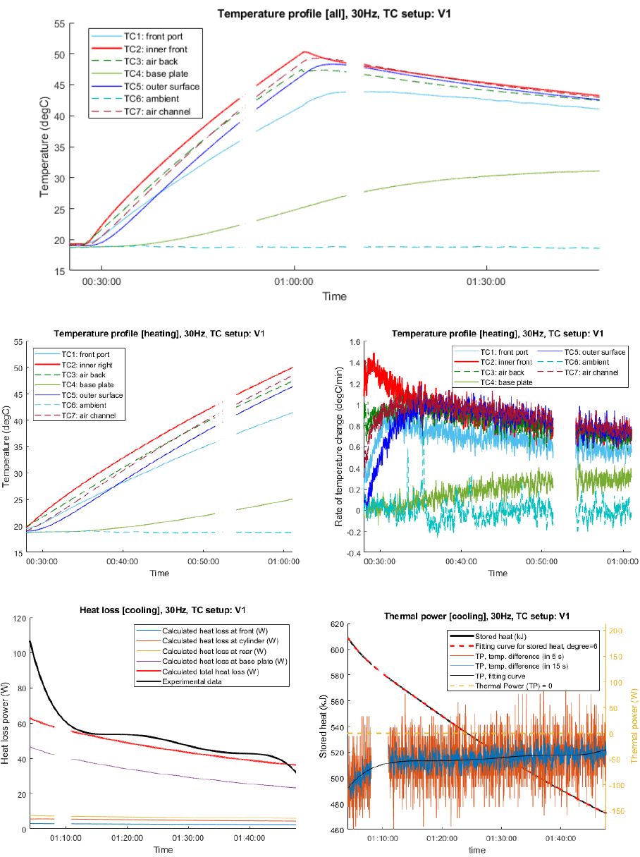
174
Figure A.9: Experiment results of 30Hz test for heat loss estimation. Several data collection
interruption at 45 min and 1 hour 10 min due to the unstable connection to the data logger and
software.

175
Figure A.10: Experiment results of 20 Hz test for heat loss estimation. The ambient temperature
was dropped at 5 hour due to the main door of lab was open for few minutes.

176
Figure A.11: The temperature readings and calculated temperature of the gap filler in the
heating phase of constant frequency tests. The temperature of gap filler was 3.1°C, 2.3°C, 1.3°C
and 0.4°C higher than the temperature of TC 2 in the test of 40, 35, 30 and 20 Hz, respectively.

177
A.8 Characteristics of induction motors
The rotational speed of an induction motor can be calculated by the following equation [275]:
(A.15)
where is rotational speed (RPM), is the primary frequency (Hz), is number of motor
poles, is slip (%). The motor efficiency is the function of the motor load and motor power.
The curves of electric motor load and efficiency is shown in Figure A.12. It can be observed
that the motor efficiency drops when the motor load is less than 40%.
Figure A.12: Electric motor part-load efficiency (as a function of full-load efficiency) [276].

178
A.9 Experimental results – core temperature measurement
Figure A.13: Experiment results of 40 Hz test with stops at TC 2 at 25, 35, 45 and 55°C.

179
Figure A.14: Experiment results of 30 Hz test with stops at TC2 at 25, 35, 45 and 55°C.

180
A.10 Others information of about proof-of-concept heater
Table A.10: Material cost of the proof-of-concept eddy current heater.
Component
Description
Cost
Baseplate
Aluminium 500x220x15mm
£50.00
End Plates
Stainless Steel (316) 220x200x20mm
£236.74
Cooling Plate
Aluminium Flange 180mmØ x 20mm
£15.00
Outer Cover
Stainless Steel Tube 8" OD, 7" ID x 9" long
£390.53
Fins (x32)
Copper 214 x 23 x 3mm
£70.00
Fin Tube
Stainless Steel Tube 5 1/2" OD, 4" ID x 9" long
£293.76
Magnet Plates (x16)
Stainless Steel 200 x 12 x 3mm
£10.00
Magnet Shaft
Stainless Steel Bar 72Ø x 210mm
£86.83
Centre Shaft
Stainless Steel Bar 30Ø x 300mm
£37.44
Bearings (x2)
SKF 62x30x16
£14.22
Oilite Bush
HPCQM303520
£6.82
Fasteners
Stainless Steel fasteners x 150
£19.52
Total material cost
£1,230.86
Table A.11: Material properties of the proof-of-concept eddy current heater [131].
Unit
Stainless
steel (316)
Aluminium
Copper
Sm
2
Co
17
Air
(1 bar)
density
kg/m3
7990
2700
8960
8400
1.28
Specific heat capacity
J/kg.K
510
910
390
370
1006
Thermal conductivity
W/m.K
15
237
401
10
0.027
Thermal expansion
10
-6
/K
16.5
24.0
16.5
8.5
3690
Table A.12: Properties of permeant magnets [277].
Properties
Value
Material
Sm
2
Co
17
(26/20)
Supplier
MAGDEV LTD.
Remanence (Br)
1.05-1.11 T
Coercivity (bHc)
744-824 kA/m
Intrinsic Coercivity (jHc)
>1440 kA/m
Max Energy Product (Bhmax)
>200 kJ/m
3
Working temperature
300°C
181
B. APPENDIX: DIRECT WIND-TO-HEAT SYSTEM FOR
ELECTRICITY GENERATION
B.1 Algorithm of searching output target for output firming
An algorithm to find the output target for output smoothing is explained. First, the initial value
of
is given and a variable , which is used to mark the state of the searching, is
set as zero. Secondly, the stored energy in the forecast horizon is calculated from time to
. If the state of storage reaches upper or lower limitations, the searching process is
interrupted and starts over with a new output target. The new output target and value of
are updated based on the state of storage:
• If the storage is not enough to store the excess power, set and increase output
target (to reduce the energy to be stored).
• If stored energy is not enough to maintain the system target, set and the
decreases output target (to increase the energy stored).
The searching process is ended if the calculation in forecast horizon is completed or the state
of storage reaches both upper and lower limitations in a searching run. The latest
is
saved as the optimal output target and used to calculate the charging or discharging power in
equation (4.6). A problem of optimising the operation based on forecast horizon is that the
system might have inefficient operations when the low or high wind generation periods are
longer than forecast horizon, such as discharging when wind power is high and charging when
wind power is low. The upper (
) and lower (
) limits of output target are applied to
prevent this unnecessary actions and the values are obtained by running a pre-simulation
without upper/lower limits, and the 75
th
and 25
th
percentile of system output are used as the
upper and lower limits, respectively.

182
Figure B.1: Algorithm of searching output target for output smoothing.

183
An example of
searching process for a system with 5 MWh stored energy is shown in
Figure B.2. In the first run of searching, the output target is set at 2.5 MW and the stored energy
is not enough to maintain the output power at . The value of is updated to -1. In the
second run, the
is reduced to 2.0 MW but still cannot maintain the output at . In
the third run, the
is reduced to 1.8 MW, the stored energy become zero at and
over storage capacity at . The searching process ends because lower and upper limits
are reached in first and third runs of searching.
Figure B.2: Example of searching system output target for capacity firming.

184
C. APPENDIX: DIRECT WIND-TO-HEAT SYSTEM FOR
HEATING
C.1 Supplementary information
Table C.1: The range of maximum temperature for process heating in different industries
[278].
Industry type
Maximum temperature range (°C)
Food processing
121 – 127
Synthetic and natural cloth processing
119 – 316
Pulp and paper processing
121 – 284
Chemical processing
110 – 427
Plastics and resins processing
188 – 274
Synthetic rubber processing
110 – 216
Metals processing
121–217
Machinery/equipment manufacturing
160 – 177
Table C.2: Solid-gas thermochemical storage candidates [164].
Type
Alkaline
Hydroxides
Alkaline
Carbonates
Metal Oxides
Chemical
Looping
Element
Ca, Sr, Ba
Ca, Sr, Ba, Mg
Co, Mn, Ba, Cu
Fe, Ni, Co, Mn
Charging
temperature (°C)
600–700
930–1400
905–1100
800–1100
Discharging
temperature (°C)
505–525
550–1300
650–900
850–950
Energy density
(kWh/m3)
22–28
5–14
9–31
38–86

185
Figure C.1: the hydrogen pipeline cost with different outer diameter and sources [251].
Figure C.2: the cost of compressed gas storage for hydrogen storage [252].

186
C.2 Calcium hydration reaction for long-term storage
The analysis of material and energy balance of calcium hydration reaction in this section is the
author’s work and published in [165]. A 10-MW of calcium hydration as thermochemical
energy storage with fluidised bed reactors is investigated.
Figure C.3: Dehydration of calcium hydroxide of a 10-MW reactor [165].
Figure C.3 shows the process diagram of a standard charging process. Calcium hydroxide at
350°C is fed into the reactor and dehydrated by a heat source (e.g. electrical heating or high-
temperature HTF) with the power of 16.6 MJ/s. Calcium oxide leaves the other end of the reactor
at 600°C. Nitrogen gas is selected as the fluidisation medium (FM) and flows into the reactor at
350°C and leaves the reactor at 600°C with the water vapour produced in the dehydration
reaction. The outlet of FM contents 7 MJ/s of thermal energy, which accounts for 42% of the
input energy. A heat exchanger can reuse the high-temperature heat in FM to heat the FM and
replace a part of the heat source. This can reduce the input heat by 2.0 MJ/s, based on a 25°C
temperature difference. The charging efficiency is about 67% based on the following equation:
(C.1)
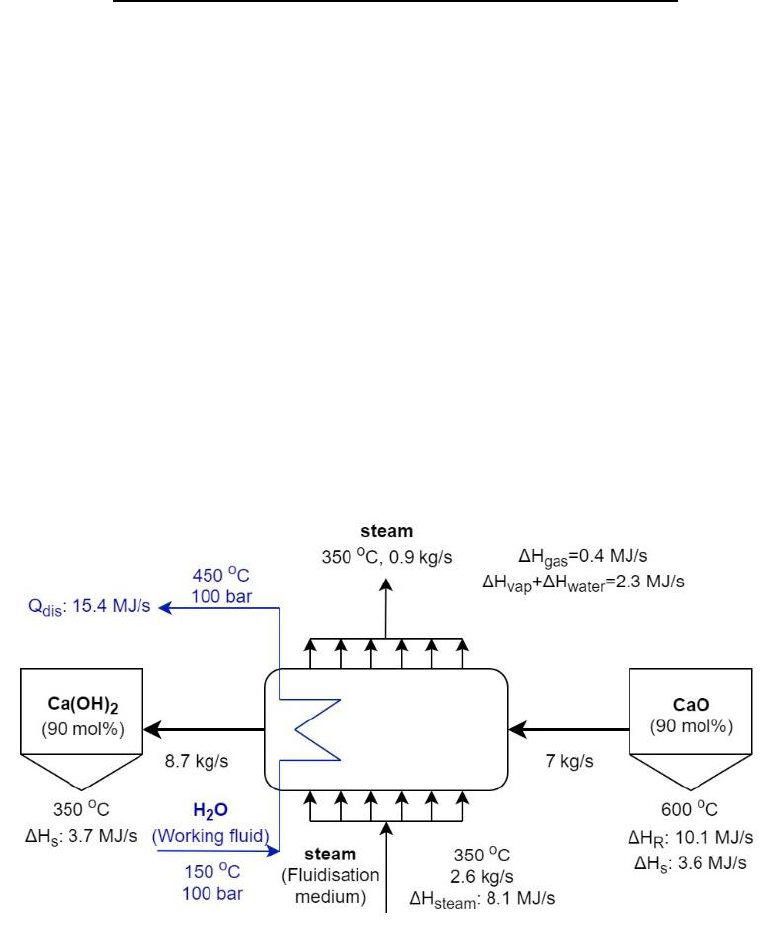
187
For long-term storage, it is desired to store calcium oxide and calcium hydroxide in ambient
temperature to minimise the heat loss from sensible heat. To keep the reactant at the same inlet
temperature, 3.7 MJ/s of heat is needed to preheat calcium hydration to 350°C. Additional heat
exchangers can reduce the energy stored in sensible heat by using the sensible heat in the outlet
material of reactor to preheat the inlet material of the reactor. This can potentially recover 3.3
MJ/s of heat based on 50°C temperature difference.
Most of the waste heat in the charging process is in the vaporisation heat of steam (3.9 MJ/s).
The charging efficiency can be further improved to 80% if 70% of the vaporisation heat can be
stored in low-temperature TES and reused later, such as TCS has charging temperature less than
100°C [163].
Figure C.4: Hydration of calcium oxide in a 10-MW fluidised bed reactor.
The discharging process is shown in Figure C.4. 350°C of steam is worked as both FM and
reactant that feeds into the reactor and reacted with calcium oxide to produce calcium hydration.
Pressurised water (150°C and 100 bar) flows into the reactor as working fluid to carry out the
generated heat as superheated steam at 450°C. FM and solid reactant leave the reactor at 350°C.
About 65% of the steam in FM is consumed in the reaction, therefore the residual heat (2.7
MJ/s) is much less than the charging process. Most of the residual heat can be reused by
preheating FM or working fluid, thus, the energy loss in the discharging process is low.
188
Because the storage material is stored in ambient temperature and pressure, the material can be
stored in standard shipping containers and its cost (0.19 £/kWh for a Twenty-foot Equivalent
Unit, TEU), which is much lower than the container for storing solid materials in high
temperature (4.5 £/kWh [164]).
189
REFERENCES
[1] IPCC, “2018: Summary for Policymakers,” 2018.
[2] Energy & Climate Intelligence Unit, “Countdown to zero,” 2019.
[3] Energy & Climate Intelligence Unit, “Net Zero Tracker.” [Online]. Available:
https://eciu.net/netzerotracker. [Accessed: 25-Feb-2020].
[4] P. Palensky and D. Dietrich, “Demand Side Management: Demand Response, Intelligent
Energy Systems, and Smart Loads,” IEEE Trans. Ind. Informatics, vol. 7, no. 3, pp. 381–
388, Aug. 2011.
[5] G. Strbac, “Demand side management: Benefits and challenges,” Energy Policy, vol. 36,
no. 12, pp. 4419–4426, Dec. 2008.
[6] E. Pean, M. Pirouti, and M. Qadrdan, “Role of the GB-France electricity interconnectors
in integration of variable renewable generation,” Renew. Energy, vol. 99, pp. 307–314,
Dec. 2016.
[7] R. A. Rodríguez, S. Becker, G. B. Andresen, D. Heide, and M. Greiner, “Transmission
needs across a fully renewable European power system,” Renew. Energy, vol. 63, pp.
467–476, Mar. 2014.
[8] European Commission, “Study on energy storage - contribution to the security of the
electricity supply in Europe,” 2020.
[9] M. McPherson and S. Tahseen, “Deploying storage assets to facilitate variable renewable
energy integration: The impacts of grid flexibility, renewable penetration, and market
structure,” Energy, vol. 145, pp. 856–870, Feb. 2018.
[10] S. Ould Amrouche, D. Rekioua, T. Rekioua, and S. Bacha, “Overview of energy storage
in renewable energy systems,” Int. J. Hydrogen Energy, vol. 41, no. 45, pp. 20914–
20927, Dec. 2016.
[11] Committee on Climate Change, “Net Zero: The UK’s contribution to stopping global
warming,” 2019.
[12] Transport & Environment, “Roadmap to decarbonising European aviation,” 2018.
[13] S. D. Watson, K. J. Lomas, and R. A. Buswell, “Decarbonising domestic heating: What
is the peak GB demand?,” Energy Policy, vol. 126, pp. 533–544, Mar. 2019.
[14] E. Williams, E. Hittinger, R. Carvalho, and R. Williams, “Wind power costs expected to
decrease due to technological progress,” Energy Policy, vol. 106, pp. 427–435, Jul. 2017.
[15] W. W. E. Association, “Wind Power Capacity Worldwide Reaches 597 GW, 50,1 GW
added in 2018,” 2019. [Online]. Available: https://wwindea.org/blog/2019/02/25/wind-
power-capacity-worldwide-reaches-600-gw-539-gw-added-in-2018/. [Accessed: 23-
Feb-2020].
[16] M. Z. Jacobson and C. L. Archer, “Saturation wind power potential and its implications
for wind energy,” Proc. Natl. Acad. Sci., vol. 109, no. 39, pp. 15679–15684, Sep. 2012.
[17] S. Cavazzi and A. G. Dutton, “An Offshore Wind Energy Geographic Information
System (OWE-GIS) for assessment of the UK’s offshore wind energy potential,” Renew.
Energy, vol. 87, no. 2016, pp. 212–228, 2016.
190
[18] National Grid ESO, “Future Energy Scenarios,” 2020.
[19] Energy System Catapult, “Innovating to net zero,” 2020.
[20] D. Nock, V. Krishnan, and J. D. McCalley, “Dispatching intermittent wind resources for
ancillary services via wind control and its impact on power system economics,” Renew.
Energy, vol. 71, pp. 396–400, Nov. 2014.
[21] Y. Scholz, H. C. Gils, and R. C. Pietzcker, “Application of a high-detail energy system
model to derive power sector characteristics at high wind and solar shares,” Energy
Econ., vol. 64, pp. 568–582, May 2017.
[22] S. Pfenninger and I. Staffell, “Long-term patterns of European PV output using 30 years
of validated hourly reanalysis and satellite data,” Energy, vol. 114, pp. 1251–1265, Nov.
2016.
[23] I. Staffell and S. Pfenninger, “Using bias-corrected reanalysis to simulate current and
future wind power output,” Energy, vol. 114, pp. 1224–1239, Nov. 2016.
[24] S. Pfenninger and I. Staffell, “Renewables Ninja.” [Online]. Available:
https://www.renewables.ninja. [Accessed: 01-Jul-2018].
[25] D. Barbosa de Alencar, C. de Mattos Affonso, R. Limão de Oliveira, J. Moya Rodríguez,
J. Leite, and J. Reston Filho, “Different Models for Forecasting Wind Power Generation:
Case Study,” Energies, vol. 10, no. 12, p. 1976, Nov. 2017.
[26] G. Giebel and G. Kariniotakis, “Wind power forecasting—a review of the state of the
art,” in Renewable Energy Forecasting, Elsevier, 2017, pp. 59–109.
[27] Q. Wang, H. Wu, A. R. Florita, C. Brancucci Martinez-Anido, and B.-M. Hodge, “The
value of improved wind power forecasting: Grid flexibility quantification, ramp
capability analysis, and impacts of electricity market operation timescales,” Appl.
Energy, vol. 184, pp. 696–713, Dec. 2016.
[28] Wind Europe, “Wind energy in Europe in 2018 - Trends and statistics,” 2019.
[29] “G.B. National Grid Status.” [Online]. Available: http://www.gridwatch.templar.co.uk/.
[Accessed: 23-Feb-2020].
[30] S. D. Ahmed, F. S. M. Al-Ismail, M. Shafiullah, F. A. Al-Sulaiman, and I. M. El-Amin,
“Grid Integration Challenges of Wind Energy: A Review,” IEEE Access, vol. 8, pp.
10857–10878, 2020.
[31] T. R. Ayodele, A. A. Jimoh, J. L. Munda, and J. T. Agee, “Challenges of grid integration
of wind power on power system grid integrity: A review,” Int. J. Renew. Energy Res.,
vol. 2, no. 4, pp. 618–626, 2012.
[32] V. Kumar, A. S. Pandey, and S. K. Sinha, “Grid integration and power quality issues of
wind and solar energy system: A review,” in 2016 International Conference on
Emerging Trends in Electrical Electronics & Sustainable Energy Systems (ICETEESES),
2016, pp. 71–80.
[33] L. Bird, M. Milligan, and D. Lew, “Integrating Variable Renewable Energy: Challenges
and Solutions,” Golden, CO (United States), Sep. 2013.
[34] G. Papaefthymiou and K. Dragoon, “Towards 100% renewable energy systems:
Uncapping power system flexibility,” Energy Policy, vol. 92, pp. 69–82, May 2016.
191
[35] M. I. Alizadeh, M. Parsa Moghaddam, N. Amjady, P. Siano, and M. K. Sheikh-El-
Eslami, “Flexibility in future power systems with high renewable penetration: A review,”
Renew. Sustain. Energy Rev., vol. 57, pp. 1186–1193, May 2016.
[36] H. Kondziella and T. Bruckner, “Flexibility requirements of renewable energy based
electricity systems – a review of research results and methodologies,” Renew. Sustain.
Energy Rev., vol. 53, pp. 10–22, Jan. 2016.
[37] M. A. Gonzalez-Salazar, T. Kirsten, and L. Prchlik, “Review of the operational
flexibility and emissions of gas- and coal-fired power plants in a future with growing
renewables,” Renew. Sustain. Energy Rev., vol. 82, pp. 1497–1513, Feb. 2018.
[38] O. de Q. F. Araújo and J. L. de Medeiros, “Carbon capture and storage technologies:
present scenario and drivers of innovation,” Curr. Opin. Chem. Eng., vol. 17, pp. 22–34,
Aug. 2017.
[39] A. Cappelletti and F. Martelli, “Investigation of a pure hydrogen fueled gas turbine
burner,” Int. J. Hydrogen Energy, vol. 42, no. 15, pp. 10513–10523, Apr. 2017.
[40] M. Ditaranto, T. Heggset, and D. Berstad, “Concept of hydrogen fired gas turbine cycle
with exhaust gas recirculation: Assessment of process performance,” Energy, vol. 192,
p. 116646, Feb. 2020.
[41] H. Jabir, J. Teh, D. Ishak, and H. Abunima, “Impacts of Demand-Side Management on
Electrical Power Systems: A Review,” Energies, vol. 11, no. 5, p. 1050, Apr. 2018.
[42] A. Kies, B. Schyska, and L. von Bremen, “The Demand Side Management Potential to
Balance a Highly Renewable European Power System,” Energies, vol. 9, no. 11, p. 955,
Nov. 2016.
[43] E. Denny et al., “The impact of increased interconnection on electricity systems with
large penetrations of wind generation: A case study of Ireland and Great Britain,” Energy
Policy, vol. 38, no. 11, pp. 6946–6954, Nov. 2010.
[44] A. Foster, “UK Interconnector Development.” National Grid, 2015.
[45] H. Chen, T. N. Cong, W. Yang, C. Tan, Y. Li, and Y. Ding, “Progress in electrical energy
storage system: A critical review,” Prog. Nat. Sci., vol. 19, no. 3, pp. 291–312, Mar.
2009.
[46] M. Beaudin, H. Zareipour, A. Schellenberglabe, and W. Rosehart, “Energy storage for
mitigating the variability of renewable electricity sources: An updated review,” Energy
Sustain. Dev., vol. 14, no. 4, pp. 302–314, Dec. 2010.
[47] International Energy Agency, “Status of Power System Transformation 2018,” 2018.
[48] H. Zhao, Q. Wu, S. Hu, H. Xu, and C. N. Rasmussen, “Review of energy storage system
for wind power integration support,” Appl. Energy, vol. 137, pp. 545–553, Jan. 2015.
[49] M.-A. Hessami and D. R. Bowly, “Economic feasibility and optimisation of an energy
storage system for Portland Wind Farm (Victoria, Australia),” Appl. Energy, vol. 88, no.
8, pp. 2755–2763, Aug. 2011.
[50] L. S. Vargas, G. Bustos-Turu, and F. Larrain, “Wind Power Curtailment and Energy
Storage in Transmission Congestion Management Considering Power Plants Ramp
Rates,” IEEE Trans. Power Syst., vol. 30, no. 5, pp. 2498–2506, Sep. 2015.
192
[51] D. M. Greenwood, K. Y. Lim, C. Patsios, P. F. Lyons, Y. S. Lim, and P. C. Taylor,
“Frequency response services designed for energy storage,” Appl. Energy, vol. 203, pp.
115–127, Oct. 2017.
[52] E. Drury, P. Denholm, and R. Sioshansi, “The value of compressed air energy storage in
energy and reserve markets,” Energy, vol. 36, no. 8, pp. 4959–4973, Aug. 2011.
[53] T. A. Nguyen and R. H. Byrne, “Maximizing the cost-savings for time-of-use and net-
metering customers using behind-the-meter energy storage systems,” in 2017 North
American Power Symposium (NAPS), 2017, pp. 1–6.
[54] H. Lund and W. Kempton, “Integration of renewable energy into the transport and
electricity sectors through V2G,” Energy Policy, vol. 36, no. 9, pp. 3578–3587, Sep.
2008.
[55] T. Okazaki and T. Nakamura, “Wind-powered thermal power generation system,”
US20150192109A1, 2015.
[56] T. Okazaki, Y. Shirai, and T. Nakamura, “Concept study of wind power utilizing direct
thermal energy conversion and thermal energy storage,” Renew. Energy, vol. 83, pp.
332–338, 2015.
[57] K. K. Cao, A. N. Nitto, E. Sperber, and A. Thess, “Expanding the horizons of power-to-
heat: Cost assessment for new space heating concepts with Wind Powered Thermal
Energy Systems,” Energy, vol. 164, pp. 925–936, 2018.
[58] D. A. Baharoon, H. A. Rahman, W. Z. W. Omar, and S. O. Fadhl, “Historical
development of concentrating solar power technologies to generate clean electricity
efficiently – A review,” Renew. Sustain. Energy Rev., vol. 41, pp. 996–1027, Jan. 2015.
[59] E. Guelpa and V. Verda, “Thermal energy storage in district heating and cooling systems:
A review,” Appl. Energy, vol. 252, p. 113474, Oct. 2019.
[60] T. Tudorache, L. Melcescu, and M. Predescu, “Analysis of a permanent magnet Eddy
current heater driven by a wind turbine,” Adv. Electr. Comput. Eng., vol. 15, no. 3, pp.
53–58, 2015.
[61] T. Watanabe, T. Todaka, and M. Enokizono, “Analysis of a new induction heating device
by using permanent magnets,” IEEE Trans. Magn., vol. 41, no. 5, pp. 1884–1887, 2005.
[62] T. Tudorache and L. Melcescu, “Outer rotor eddy current heater for wind turbines,”
Renew. Energy Environ. Sustain., vol. 1, p. 25, 2016.
[63] O. Nebi and V. Fireteanu, “Finite element analysis of an eddy currents heater for wind
or water kinetic energy conversion into heat,” in Renewable Energy and Power Quality
Journal, 2010, vol. 1, no. 08, pp. 882–887.
[64] T. Tudorache and M. Popescu, “FEM optimal design of wind energy-based heater,” Acta
Polytech. Hungarica, vol. 6, no. 2, pp. 55–70, 2009.
[65] V. Fireteanu and O. Nebi, “Finite Element Electromagnetic 2D Model of an Eddy,” no.
32, pp. 62–67, 2008.
[66] I. Sobor, V. Rachier, A. Chiciuc, and Rodion Ciuperca, “Small Wind Energy System
With Permanent Magnet Eddy Current Heater,” no. Lxiii, 2013.
[67] L. Chen, Y. Pei, F. Chai, and S. Cheng, “Investigation of a Novel Mechanical to Thermal
193
Energy Converter Based on the Inverse Problem of Electric Machines,” Energies, vol.
9, no. 7, p. 518, 2016.
[68] T. Okazaki, T. Matsuo, and T. Mifune, “Induction heating apparatus and power
generation system comprising the same,” US20140110938A1, 2014.
[69] T. Okazaki, “Electric power generation system,” US20160252076A1, 2016.
[70] T. Matsuo and T. Okazaki, “A Basic Theory of Induction Heating for a Wind-Powered
Thermal Energy System,” IEEE Trans. Magn., vol. 53, no. 11, 2017.
[71] O. Dumont, G. F. Frate, A. Pillai, S. Lecompte, M. De paepe, and V. Lemort, “Carnot
battery technology: A state-of-the-art review,” J. Energy Storage, vol. 32, p. 101756,
Dec. 2020.
[72] W.-D. Steinmann, H. Jockenhöfer, and D. Bauer, “Thermodynamic Analysis of High‐
Temperature Carnot Battery Concepts,” Energy Technol., vol. 8, no. 3, p. 1900895, Mar.
2020.
[73] S. D. Garvey et al., “On generation-integrated energy storage,” Energy Policy, vol. 86,
pp. 544–551, 2015.
[74] S. D. Garvey et al., “Analysis of a Wind Turbine Power Transmission System with
Intrinsic Energy Storage Capability,” Wind Eng., vol. 39, no. 2, pp. 149–173, Apr. 2015.
[75] S. D. Garvey, “Integrating Energy Storage with Renewable Energy Generation,” Wind
Eng., vol. 39, no. 2, pp. 129–140, 2015.
[76] G. Jose and R. Chacko, “A review on wind turbine transformers,” in 2014 Annual
International Conference on Emerging Research Areas: Magnetics, Machines and
Drives (AICERA/iCMMD), 2014, pp. 1–7.
[77] S. M. Muyeen, Ed., “Chapter 2 Calculation Method of Losses and Efficiency of Wind
Generators,” in Wind Energy Conversion Systems, 2012.
[78] H. Polinder, F. F. A. Van Der Pijl, G. J. De Vilder, and P. J. Tavner, “Comparison of
direct-drive and geared generator concepts for wind turbines,” IEEE Trans. Energy
Convers., vol. 21, no. 3, pp. 725–733, 2006.
[79] M. D. Reder, E. Gonzalez, and J. J. Melero, “Wind Turbine Failures - Tackling current
Problems in Failure Data Analysis,” J. Phys. Conf. Ser., vol. 753, no. 7, 2016.
[80] P. Jaen-Sola, A. S. McDonald, and E. Oterkus, “Lightweight design of direct-drive wind
turbine electrical generators: A comparison between steel and composite material
structures,” Ocean Eng., vol. 181, pp. 330–341, Jun. 2019.
[81] J. G. Manwell, A. L. McGowan, and J. F. Rogers, Wind energy explained, Second Edi.,
vol. 3, no. 3. Wiley, 2009.
[82] R. Wailes, “Horizontal Windmills,” Trans. Newcom. Soc., vol. XL, pp. 125–145, 1967.
[83] International Energy Agency, “IEA - Data and statistics.” [Online]. Available:
https://www.iea.org/data-and-statistics. [Accessed: 20-Feb-2020].
[84] P. J. Schubel and R. J. Crossley, “Wind Turbine Blade Design,” Energies, vol. 5, no. 9,
pp. 3425–3449, Sep. 2012.
[85] E. Hau and H. von Renouard, Wind Turbines. Berlin, Heidelberg: Springer Berlin
194
Heidelberg, 2006.
[86] M. Ragheb, “Optimal Rotor Tip Speed Ratio,” Work. Notes, pp. 1–10, 2009.
[87] J. F. Manwell and J. G. McGowan, “A design procedure for wind powered heating
systems,” Sol. Energy, vol. 26, no. 5, pp. 437–445, 1981.
[88] B. Ashikian, “Wind motor operated heating system,” US3752395A, 1971.
[89] U. Hansen, “Wind powered heating circuit - has sails on wind tower driving eddy current
brake for producing heat for heat exchange fluid,” DE2901997A1, 1980.
[90] J. T. Hamrick and L. C. Rose, “Heat pump operated by wind or other power means,”
US4304103A, 1980.
[91] “H2o Turines.” [Online]. Available: https://www.h2oturbines.com/about. [Accessed:
19-Feb-2020].
[92] K. De Decker, “Heat your House with a Mechanical Windmill,” LOW-TECH
MAGAZINE, 2019. [Online]. Available:
https://www.lowtechmagazine.com/2019/02/heat-your-house-with-a-water-brake-
windmill.html. [Accessed: 28-Sep-2020].
[93] BEIS (Department for Business Energy & Industrial Strategy), “Quarterly Energy Prices:
December 2019,” 2019.
[94] A. Hepbasli and Y. Kalinci, “A review of heat pump water heating systems,” Renew.
Sustain. Energy Rev., vol. 13, no. 6–7, pp. 1211–1229, Aug. 2009.
[95] S. M. Sami, E. E. Wilson, D. J. Bratel, and J. H. Batten, “Power generator using a wind
turbine, a hydrodynamic retarder and an organic Rankine cycle drive,”
US20120001436A1, 2012.
[96] J. L. Lee, “On-demand generation of electricity from stored wind energy,”
US20120326445A1, 2012.
[97] B. F. Tchanche, G. Lambrinos, A. Frangoudakis, and G. Papadakis, “Low-grade heat
conversion into power using organic Rankine cycles – A review of various applications,”
Renew. Sustain. Energy Rev., vol. 15, no. 8, pp. 3963–3979, Oct. 2011.
[98] P. C. Verma, R. Ciudin, A. Bonfanti, P. Aswath, G. Straffelini, and S. Gialanella, “Role
of the friction layer in the high-temperature pin-on-disc study of a brake material,” Wear,
vol. 346–347, pp. 56–65, Jan. 2016.
[99] H. Jang, K. Ko, S. . Kim, R. . Basch, and J. . Fash, “The effect of metal fibers on the
friction performance of automotive brake friction materials,” Wear, vol. 256, no. 3–4,
pp. 406–414, Feb. 2004.
[100] Y. V. Roustiam Chakirov, “Direct Conversion of Wind Energy into Heat Using Joule
Machine,” Int. Conf. Environ. Comput. Sci., vol. 19, pp. 12–17, 2011.
[101] T. Zdankus, J. Cerneckiene, A. Jurelionis, and J. Vaiciunas, “Experimental study of a
small scale hydraulic system for mechanical wind energy conversion into heat,” Sustain.,
vol. 8, no. 7, 2016.
[102] C. Y. Liu, K. J. Jiang, and Y. Zhang, “Design and use of an eddy current retarder in an
automobile,” Int. J. Automot. Technol., vol. 12, no. 4, pp. 611–616, Aug. 2011.
195
[103] J. Tian, D. Li, K. Ning, and L. Ye, “Research on Heat Dissipation Optimization of a
Novel Liquid-cooling Eddy Current Brake,” IEEE Trans. Energy Convers., pp. 1–1,
2020.
[104] P. J. Wang and S. J. Chiueh, “Analysis of eddy-current brakes for high speed railway,”
IEEE Trans. Magn., vol. 34, no. 4 PART 1, pp. 1237–1239, 1998.
[105] M. Jou, J. K. Shiau, and C. C. Sun, “Design of a magnetic braking system,” J. Magn.
Magn. Mater., vol. 304, no. 1, pp. 234–236, 2006.
[106] K. J. Chua, S. K. Chou, and W. M. Yang, “Advances in heat pump systems: A review,”
Appl. Energy, vol. 87, no. 12, pp. 3611–3624, Dec. 2010.
[107] C. Arpagaus, F. Bless, M. Uhlmann, J. Schiffmann, and S. S. Bertsch, “High temperature
heat pumps: Market overview, state of the art, research status, refrigerants, and
application potentials,” Energy, vol. 152, pp. 985–1010, 2018.
[108] J. Braymer, M. Pinotti, and A. Dybbs, “A WIND POWERED HEAT PUMP,” in Energy,
Resources and Environment, Elsevier, 1982, pp. 528–535.
[109] C.-S. Jwo, Z.-J. Chien, Y.-L. Chen, and C.-C. Chien, “Development of a Wind Directly
Forced Heat Pump and Its Efficiency Analysis,” Int. J. Photoenergy, vol. 2013, pp. 1–7,
2013.
[110] J. D. McTigue, A. J. White, and C. N. Markides, “Parametric studies and optimisation
of pumped thermal electricity storage,” Appl. Energy, vol. 137, pp. 800–811, Jan. 2015.
[111] A. Benato and A. Stoppato, “Pumped Thermal Electricity Storage: A technology
overview,” Therm. Sci. Eng. Prog., vol. 6, pp. 301–315, Jun. 2018.
[112] IRENA, “Renewable energy technologies: cost analysis series - Concentrating Solar
Power,” 2012.
[113] BEIS, “Electricity Generation Costs,” 2016.
[114] K. Vignarooban, X. Xu, A. Arvay, K. Hsu, and A. M. Kannan, “Heat transfer fluids for
concentrating solar power systems - A review,” Appl. Energy, vol. 146, pp. 383–396,
2015.
[115] H. Benoit, L. Spreafico, D. Gauthier, and G. Flamant, “Review of heat transfer fluids in
tube-receivers used in concentrating solar thermal systems: Properties and heat transfer
coefficients,” Renew. Sustain. Energy Rev., vol. 55, pp. 298–315, 2016.
[116] E. Bellos, C. Tzivanidis, K. A. Antonopoulos, and I. Daniil, “The use of gas working
fluids in parabolic trough collectors – An energetic and exergetic analysis,” Appl. Therm.
Eng., vol. 109, pp. 1–14, 2016.
[117] N. Lorenzin and A. Abánades, “A review on the application of liquid metals as heat
transfer fluid in Concentrated Solar Power technologies,” Int. J. Hydrogen Energy, vol.
41, no. 17, pp. 6990–6995, 2016.
[118] H. Lund et al., “4th Generation District Heating (4GDH). Integrating smart thermal grids
into future sustainable energy systems.,” Energy, vol. 68, pp. 1–11, 2014.
[119] E. Bellos, C. Tzivanidis, and K. A. Antonopoulos, “A detailed working fluid
investigation for solar parabolic trough collectors,” Appl. Therm. Eng., vol. 114, pp. 374–
386, 2017.
196
[120] Wind directions, “Supply Chain: The Race to meet Demand,” Wind Directions, no.
January/February, pp. 27–34, 2007.
[121] A. R. Hambley, Electrical Engineering - Principles and Applications, Sixth edit.
Pearson.
[122] M. I. González, “Experiments with eddy currents: the eddy current brake,” Eur. J. Phys.,
vol. 25, no. 4, pp. 463–468, Jul. 2004.
[123] H.-J. Shin, J.-Y. Choi, H.-W. Cho, and S.-M. Jang, “Analytical Torque Calculations and
Experimental Testing of Permanent Magnet Axial Eddy Current Brake,” IEEE Trans.
Magn., vol. 49, no. 7, pp. 4152–4155, Jul. 2013.
[124] S. E. Gay and M. Ehsani, “Parametric analysis of eddy-current brake performance by 3-
D finite-element analysis,” IEEE Trans. Magn., vol. 42, no. 2, pp. 319–328, Feb. 2006.
[125] Chetvorno, “Eddy current brake diagram,” 2015. [Online]. Available:
https://commons.wikimedia.org/wiki/File:Eddy_current_brake_diagram.svg.
[Accessed: 02-Oct-2020].
[126] H. Polinder, M. J. Hoeijmakers, and M. Scuotto, “Eddy-Current Losses in the Solid
Back-Iron of PM Machines for different Concentrated Fractional Pitch Windings,” in
2007 IEEE International Electric Machines & Drives Conference, 2007, pp. 652–657.
[127] T. A. Short, Electric power distribution handbook. CRC Press, 2003.
[128] S. R. Trout, “Material selection of permanent magnets, considering thermal properties
correctly,” in Proceedings: Electrical Insulation Conference and Electrical
Manufacturing and Coil Winding Conference (Cat. No.01CH37264), pp. 365–370.
[129] Glenn Research Center, “High-temperature Coils for Electromagnets,” Tech Briefs,
2002. [Online]. Available:
https://www.techbriefs.com/component/content/article/tb/techbriefs/electronics-and-
computers/6887. [Accessed: 29-Jan-2020].
[130] MAGDEV LTD, “Permanent magnet - material selection guide.” [Online]. Available:
https://www.magdev.co.uk/material-selection-guide. [Accessed: 29-Jan-2020].
[131] MatWeb, “Material Property Data.” [Online]. Available: http://www.matweb.com.
[Accessed: 10-Oct-2019].
[132] “The Engineering ToolBox.” [Online]. Available:
https://www.engineeringtoolbox.com/. [Accessed: 30-Jan-2020].
[133] H. A. Wheeler, “Formulas for the Skin Effect,” Proc. IRE, vol. 30, no. 9, pp. 412–424,
Sep. 1942.
[134] K. C. Kavvadias and S. Quoilin, “Exploiting waste heat potential by long distance heat
transmission: Design considerations and techno-economic assessment,” Appl. Energy,
vol. 216, no. November 2017, pp. 452–465, 2018.
[135] I. Sarbu and C. Sebarchievici, “A Comprehensive Review of Thermal Energy Storage,”
Sustainability, vol. 10, no. 2, p. 191, Jan. 2018.
[136] C. A. Cruickshank and S. J. Harrison, “Heat loss characteristics for a typical solar
domestic hot water storage,” Energy Build., vol. 42, no. 10, pp. 1703–1710, Oct. 2010.
[137] S. Ushak, A. G. Fernández, and M. Grageda, “Using molten salts and other liquid
197
sensible storage media in thermal energy storage (TES) systems,” in Advances in
Thermal Energy Storage Systems, Elsevier, 2015, pp. 49–63.
[138] S. Ayyappan, K. Mayilsamy, and V. V. Sreenarayanan, “Performance improvement
studies in a solar greenhouse drier using sensible heat storage materials,” Heat Mass
Transf., vol. 52, no. 3, pp. 459–467, Mar. 2016.
[139] J. Radcliffe and Y. Li, “Thermal energy storage in Scotland,” Therm. energy storage
Scotl., no. July, 2015.
[140] A. B. Gallo, J. R. Simões-Moreira, H. K. M. Costa, M. M. Santos, and E. Moutinho dos
Santos, “Energy storage in the energy transition context: A technology review,” Renew.
Sustain. Energy Rev., vol. 65, pp. 800–822, Nov. 2016.
[141] BEIS, “Evidence Gathering: Thermal Energy Storage (TES) Technologies,” 2016.
[142] A. Dahash, F. Ochs, M. B. Janetti, and W. Streicher, “Advances in seasonal thermal
energy storage for solar district heating applications: A critical review on large-scale hot-
water tank and pit thermal energy storage systems,” Appl. Energy, vol. 239, pp. 296–
315, Apr. 2019.
[143] C. Liu, M.-S. Cheng, B.-C. Zhao, and Z.-M. Dai, “A Wind Power Plant with Thermal
Energy Storage for Improving the Utilization of Wind Energy,” Energies, vol. 10, no.
12, p. 2126, Dec. 2017.
[144] N. Fitzgerald, A. M. Foley, and E. McKeogh, “Integrating wind power using intelligent
electric water heating,” Energy, vol. 48, no. 1, pp. 135–143, Dec. 2012.
[145] Siemens Gamesa, “Electric Thermal Energy Storage.” [Online]. Available:
https://www.siemensgamesa.com/en-int/products-and-services/hybrid-and-
storage/thermal-energy-storage-with-etes. [Accessed: 12-Mar-2020].
[146] “Malta Inc.” [Online]. Available: https://www.maltainc.com/. [Accessed: 28-Feb-2020].
[147] A. Sharma, V. V. Tyagi, C. R. Chen, and D. Buddhi, “Review on thermal energy storage
with phase change materials and applications,” Renew. Sustain. Energy Rev., vol. 13, no.
2, pp. 318–345, Feb. 2009.
[148] B. Ameel et al., “Thermodynamic analysis of energy storage with a liquid air Rankine
cycle,” Appl. Therm. Eng., vol. 52, no. 1, pp. 130–140, Apr. 2013.
[149] M. K. A. Sharif et al., “Review of the application of phase change material for heating
and domestic hot water systems,” Renew. Sustain. Energy Rev., vol. 42, pp. 557–568,
Feb. 2015.
[150] “The world’s first large scale composite Phase Change Material demonstration plant for
curtailed wind power.” [Online]. Available:
https://www.birmingham.ac.uk/research/energy/news/2018/worlds-first-large-scale-
composite-phase-change-material-demonstration-plant.aspx. [Accessed: 28-Feb-2020].
[151] B. Xu, P. Li, and C. Chan, “Application of phase change materials for thermal energy
storage in concentrated solar thermal power plants: A review to recent developments,”
Appl. Energy, vol. 160, pp. 286–307, 2015.
[152] E. Oró, A. de Gracia, A. Castell, M. M. Farid, and L. F. Cabeza, “Review on phase
change materials (PCMs) for cold thermal energy storage applications,” Appl. Energy,
vol. 99, pp. 513–533, Nov. 2012.
198
[153] A. CHAN, T. CHOW, S. FONG, and J. LIN, “Performance evaluation of district cooling
plant with ice storage,” Energy, vol. 31, no. 14, pp. 2750–2762, Nov. 2006.
[154] W. Lu and S. A. Tassou, “Characterization and experimental investigation of phase
change materials for chilled food refrigerated cabinet applications,” Appl. Energy, vol.
112, pp. 1376–1382, Dec. 2013.
[155] J. Lizana, R. Chacartegui, A. Barrios-Padura, and J. M. Valverde, “Advances in thermal
energy storage materials and their applications towards zero energy buildings: A critical
review,” Appl. Energy, vol. 203, pp. 219–239, Oct. 2017.
[156] P. Pardo, A. Deydier, Z. Anxionnaz-Minvielle, S. Rougé, M. Cabassud, and P. Cognet,
“A review on high temperature thermochemical heat energy storage,” Renew. Sustain.
Energy Rev., vol. 32, pp. 591–610, Apr. 2014.
[157] K. E. N’Tsoukpoe, H. Liu, N. Le Pierrès, and L. Luo, “A review on long-term sorption
solar energy storage,” Renew. Sustain. Energy Rev., vol. 13, no. 9, pp. 2385–2396, Dec.
2009.
[158] Y. Ding and S. B. Riffat, “Thermochemical energy storage technologies for building
applications: a state-of-the-art review,” Int. J. Low-Carbon Technol., vol. 8, no. 2, pp.
106–116, Jun. 2013.
[159] H. Zhang, K. Huys, J. Baeyens, J. Degrève, W. Kong, and Y. Lv, “Thermochemical
Energy Storage for Power Generation on Demand,” Energy Technol., vol. 4, no. 2, pp.
341–352, Feb. 2016.
[160] C. Prieto, P. Cooper, A. I. Fernández, and L. F. Cabeza, “Review of technology:
Thermochemical energy storage for concentrated solar power plants,” Renewable and
Sustainable Energy Reviews, vol. 60. pp. 909–929, 2016.
[161] R. Chacartegui, A. Alovisio, C. Ortiz, J. M. Valverde, V. Verda, and J. A. Becerra,
“Thermochemical energy storage of concentrated solar power by integration of the
calcium looping process and a CO<inf>2</inf> power cycle,” Appl. Energy, vol. 173,
2016.
[162] C. Chen, K. M. Lovegrove, A. Sepulveda, and A. S. Lavine, “Design and optimization
of an ammonia synthesis system for ammonia-based solar thermochemical energy
storage,” Sol. Energy, vol. 159, no. June 2017, pp. 992–1002, 2018.
[163] G. Krese, R. Koželj, V. Butala, and U. Stritih, “Thermochemical seasonal solar energy
storage for heating and cooling of buildings,” Energy Build., vol. 164, pp. 239–253,
2018.
[164] A. Bayon et al., “Techno-economic assessment of solid–gas thermochemical energy
storage systems for solar thermal power applications,” Energy, vol. 149, pp. 473–484,
2018.
[165] Y.-C. Chen, J. Radcliffe, and Y. Ding, “Concept of offshore direct wind-to-heat system
integrated with thermal energy storage for decarbonising heating,” in 2019 Offshore
Energy and Storage Summit (OSES), 2019, pp. 1–8.
[166] BEIS (Department for Business Energy & Industrial Strategy), “Energy consumption in
the UK,” 2019. [Online]. Available: https://www.gov.uk/government/statistics/energy-
consumption-in-the-uk. [Accessed: 22-Aug-2020].
199
[167] BEIS (Department for Business Energy & Industrial Strategy), “Digest of United
Kingdom Energy Statistics 2019,” 2019.
[168] DECC Statistics, “Estimates of heat use in the United Kingdom in 2013,” 2014.
[169] UK Energy REsearch Centre, “Challenges for the decarbonisation of heat: local gas
demand vs electricity supply Winter 2017/2018,” 2018.
[170] UKERC, “Flexibility in Great Britain’s gas networks: analysis of linepack and linepack
flexibility using hourly data,” 2019.
[171] BEIS (Department for Business Energy & Industrial Strategy), “Clean Growth -
Transforming Heating,” no. December, 2018.
[172] G. Strbac et al., “Analysis of Alternative UK Heat Decarbonisation Pathways For the
Committee on Climate Change,” no. June, 2018.
[173] A. Honore, “Decarbonisation of heat in Europe,” Oxford, United Kingdom, May 2018.
[174] Energy Technologies Institue, “District heat networks in the UK,” 2018.
[175] H. K. Jeswani, A. Whiting, and A. Azapagic, “Environmental and Economic
Sustainability of Biomass Heat in the UK,” Energy Technol., p. 1901044, Nov. 2019.
[176] J. O. Abe, A. P. I. Popoola, E. Ajenifuja, and O. M. Popoola, “Hydrogen energy,
economy and storage: Review and recommendation,” Int. J. Hydrogen Energy, vol. 44,
no. 29, pp. 15072–15086, Jun. 2019.
[177] ICEF, “Industrial heat decarbonisation roadmap,” 2019.
[178] C. K. Ho and B. D. Iverson, “Review of high-temperature central receiver designs for
concentrating solar power,” Renew. Sustain. Energy Rev., vol. 29, pp. 835–846, Jan.
2014.
[179] B.-J. Huang, Y.-C. Huang, G.-Y. Chen, P.-C. Hsu, and K. Li, “Improving Solar PV
System Efficiency Using One-Axis 3-Position Sun Tracking,” Energy Procedia, vol. 33,
pp. 280–287, 2013.
[180] Heat Roadmap Europe, “Heating and cooling: The transformation towrads a low-carbon
Heating & Cooling sector,” 2017.
[181] P. M. Congedo, C. Baglivo, S. Bonuso, D. D’Agostino, and D. D’Agostino, “Numerical
and experimental analysis of the energy performance of an air-source heat pump (ASHP)
coupled with a horizontal earth-to-air heat exchanger (EAHX) in different climates,”
Geothermics, vol. 87, no. April, p. 101845, Sep. 2020.
[182] Z. Abdin and W. Mérida, “Hybrid energy systems for off-grid power supply and
hydrogen production based on renewable energy: A techno-economic analysis,” Energy
Convers. Manag., vol. 196, pp. 1068–1079, Sep. 2019.
[183] L. Mosca, E. Palo, M. Colozzi, G. Iaquaniello, A. Salladini, and S. Taraschi, “Hydrogen
in chemical and petrochemical industry,” in Current Trends and Future Developments
on (Bio-) Membranes, Elsevier, 2020, pp. 387–410.
[184] D. G. Caglayan et al., “Technical potential of salt caverns for hydrogen storage in
Europe,” Int. J. Hydrogen Energy, vol. 45, no. 11, pp. 6793–6805, Feb. 2020.
[185] I. Staffell, “The Energy and Fuel Data Sheet,” 2011.
200
[186] V. Masatin, E. Latõšev, and A. Volkova, “Evaluation Factor for District Heating
Network Heat Loss with Respect to Network Geometry,” Energy Procedia, vol. 95, pp.
279–285, Sep. 2016.
[187] Q. Ma, L. Luo, R. Z. Wang, and G. Sauce, “A review on transportation of heat energy
over long distance: Exploratory development,” Renew. Sustain. Energy Rev., vol. 13, no.
6–7, pp. 1532–1540, Aug. 2009.
[188] H. Böhm and J. Lindorfer, “Techno-economic assessment of seasonal heat storage in
district heating with thermochemical materials,” Energy, vol. 179, pp. 1246–1264, 2019.
[189] W. L. Cheng, B. C. Han, Y. Le Nian, and B. B. Han, “Theoretical analysis of a wind
heating conversion and long distance transmission system,” Energy Convers. Manag.,
vol. 137, pp. 21–33, 2017.
[190] T. Nomura, N. Okinaka, and T. Akiyama, “Waste heat transportation system, using phase
change material (PCM) from steelworks to chemical plant,” Resour. Conserv. Recycl.,
vol. 54, no. 11, pp. 1000–1006, Sep. 2010.
[191] M. Angerer et al., “Design of a MW-scale thermo-chemical energy storage reactor,”
Energy Reports, vol. 4, pp. 507–519, 2018.
[192] C. E. J. Clark, R. B. Fancher, D. M. Nesbitt, and S. G. Regulinski, “Calculating the cost
of producing energy for regulated and nonregulated industry,” Los Altos, CA (USA),
1980.
[193] R. Gross, P. Heptonstall, and W. Blyth, “Investment in electricity generation: the role of
costs, incentives and risks,” 2007.
[194] C. S. Lai and M. D. McCulloch, “Levelized cost of electricity for solar photovoltaic and
electrical energy storage,” Appl. Energy, vol. 190, pp. 191–203, Mar. 2017.
[195] V. Jülch, “Comparison of electricity storage options using levelized cost of storage
(LCOS) method,” Appl. Energy, vol. 183, pp. 1594–1606, Dec. 2016.
[196] Nord Pool AS, “Nord Pool - Historical Market Data.” [Online]. Available:
https://www.nordpoolgroup.com/historical-market-data/. [Accessed: 02-Mar-2020].
[197] Lazard, “Lazard’s levelized cost of storage analysis - version 5.0,” 2019.
[198] M. Obi, S. M. M. Jensen, J. B. Ferris, and R. B. Bass, “Calculation of levelized costs of
electricity for various electrical energy storage systems,” Renew. Sustain. Energy Rev.,
vol. 67, pp. 908–920, Jan. 2017.
[199] K. Mongird et al., “Energy Storage Technology and Cost Characterization Report,”
2019.
[200] R. Dufo-López and J. L. Bernal-Agustín, “Techno-economic analysis of grid-connected
battery storage,” Energy Convers. Manag., vol. 91, pp. 394–404, Feb. 2015.
[201] F. Brahman, M. Honarmand, and S. Jadid, “Optimal electrical and thermal energy
management of a residential energy hub, integrating demand response and energy
storage system,” Energy Build., vol. 90, pp. 65–75, Mar. 2015.
[202] G. Notton et al., “Intermittent and stochastic character of renewable energy sources:
Consequences, cost of intermittence and benefit of forecasting,” Renew. Sustain. Energy
Rev., vol. 87, pp. 96–105, May 2018.
201
[203] W. Katzenstein and J. Apt, “The cost of wind power variability,” Energy Policy, vol. 51,
pp. 233–243, Dec. 2012.
[204] S. R. Sinsel, R. L. Riemke, and V. H. Hoffmann, “Challenges and solution technologies
for the integration of variable renewable energy sources—a review,” Renew. Energy,
vol. 145, pp. 2271–2285, Jan. 2020.
[205] Agora Energiewende, “The integration costs of wind and solar power,” 2014.
[206] H. Algarvio, F. Lopes, A. Couto, J. Santana, and A. Estanqueiro, “Effects of regulating
the European Internal Market on the integration of variable renewable energy,” Wiley
Interdiscip. Rev. Energy Environ., vol. 8, no. 6, Nov. 2019.
[207] A. Coester, M. W. Hofkes, and E. Papyrakis, “An optimal mix of conventional power
systems in the presence of renewable energy: A new design for the German electricity
market,” Energy Policy, vol. 116, pp. 312–322, May 2018.
[208] P. D. Myers and D. Y. Goswami, “Thermal energy storage using chloride salts and their
eutectics,” Appl. Therm. Eng., vol. 109, pp. 889–900, Oct. 2016.
[209] A. Berrada and K. Loudiyi, “Operation, sizing, and economic evaluation of storage for
solar and wind power plants,” Renew. Sustain. Energy Rev., vol. 59, pp. 1117–1129, Jun.
2016.
[210] F. de Bosio and V. Verda, “Thermoeconomic analysis of a Compressed Air Energy
Storage (CAES) system integrated with a wind power plant in the framework of the IPEX
Market,” Appl. Energy, vol. 152, pp. 173–182, Aug. 2015.
[211] S. V. Papaefthymiou and S. A. Papathanassiou, “Optimum sizing of wind-pumped-
storage hybrid power stations in island systems,” Renew. Energy, vol. 64, pp. 187–196,
Apr. 2014.
[212] S. Succar, D. C. Denkenberger, and R. H. Williams, “Optimization of specific rating for
wind turbine arrays coupled to compressed air energy storage,” Appl. Energy, vol. 96,
pp. 222–234, Aug. 2012.
[213] B. Li and J. F. DeCarolis, “A techno-economic assessment of offshore wind coupled to
offshore compressed air energy storage,” Appl. Energy, vol. 155, pp. 315–322, Oct.
2015.
[214] C. Forsberg, S. Brick, and G. Haratyk, “Coupling heat storage to nuclear reactors for
variable electricity output with baseload reactor operation,” Electr. J., vol. 31, no. 3, pp.
23–31, Apr. 2018.
[215] A. J. Pimm, S. D. Garvey, and B. Kantharaj, “Economic analysis of a hybrid energy
storage system based on liquid air and compressed air,” J. Energy Storage, vol. 4, pp.
24–35, 2015.
[216] C. Xie, Y. Hong, Y. Ding, Y. Li, and J. Radcliffe, “An economic feasibility assessment
of decoupled energy storage in the UK: With liquid air energy storage as a case study,”
Appl. Energy, vol. 225, no. February, pp. 244–257, 2018.
[217] R. Weron, “Electricity price forecasting: A review of the state-of-the-art with a look into
the future,” Int. J. Forecast., vol. 30, no. 4, pp. 1030–1081, Oct. 2014.
[218] F. Zhang and H. Fleyeh, “A Review of Single Artificial Neural Network Models for
Electricity Spot Price Forecasting,” in 2019 16th International Conference on the
202
European Energy Market (EEM), 2019, pp. 1–6.
[219] F. Zhang and H. Fleyeh, “Hybrid Artificial Neural Networks Based Models for
Electricity Spot Price Forecasting - A Review,” in 2019 16th International Conference
on the European Energy Market (EEM), 2019, pp. 1–6.
[220] H. Maeda and Y. Yanagisawa, “Recent Developments in High-Temperature
Superconducting Magnet Technology (Review),” IEEE Trans. Appl. Supercond., vol.
24, no. 3, pp. 1–12, Jun. 2014.
[221] Y.-K. Wu, C.-Z. Tsai, and Y.-H. Li, “Design of wind power generators: Summary and
comparison,” in 2018 IEEE International Conference on Applied System Invention
(ICASI), 2018, pp. 1314–1317.
[222] X. Song et al., “Experimental Validation of a Full-Size Pole Pair Set-Up of an MW-
Class Direct Drive Superconducting Wind Turbine Generator,” IEEE Trans. Energy
Convers., vol. 35, no. 2, pp. 1120–1128, Jun. 2020.
[223] R. W. Serth, Process Heat Transfer. Elsevier, 2007.
[224] A. M. Papadopoulos, “State of the art in thermal insulation materials and aims for future
developments,” Energy Build., vol. 37, no. 1, pp. 77–86, Jan. 2005.
[225] R. Baetens et al., “Vacuum insulation panels for building applications: A review and
beyond,” Energy Build., vol. 42, no. 2, pp. 147–172, Feb. 2010.
[226] M. Lämmle, T. Kroyer, S. Fortuin, M. Wiese, and M. Hermann, “Development and
modelling of highly-efficient PVT collectors with low-emissivity coatings,” Sol. Energy,
vol. 130, pp. 161–173, Jun. 2016.
[227] T. Gil-Lopez, M. A. Galvez-Huerta, J. Castejon-Navas, and V. Gomez-Garcia,
“Experimental analysis of energy savings and hygrothermal conditions improvement by
means of air curtains in stores with intensive pedestrian traffic,” Energy Build., vol. 67,
pp. 608–615, Dec. 2013.
[228] Oilite Bushes, “Shafts & Bearings.” [Online]. Available:
https://www.hpcgears.com/pdf_c33/4.14-4.19.pdf. [Accessed: 02-Feb-2020].
[229] Henkel - Adhesive Technologies, “LOCTITE AA 3342.” [Online]. Available:
https://www.henkel-adhesives.com/de/de/produkt/structural-
adhesives/loctite_aa_3342.html. [Accessed: 02-Feb-2020].
[230] P. S. Ghoshdastidar, Heat Transfer, 2nd ed. Oxford University Press, 2012.
[231] The Engineering ToolBox, “Slip in Electrical Induction Motors.” [Online]. Available:
https://www.engineeringtoolbox.com/electrical-motor-slip-d_652.html. [Accessed: 16-
Feb-2020].
[232] F. Ueckerdt et al., “Representing power sector variability and the integration of variable
renewables in long-term energy-economy models using residual load duration curves,”
Energy, vol. 90, pp. 1799–1814, Oct. 2015.
[233] F. Ueckerdt, R. Pietzcker, Y. Scholz, D. Stetter, A. Giannousakis, and G. Luderer,
“Decarbonizing global power supply under region-specific consideration of challenges
and options of integrating variable renewables in the REMIND model,” Energy Econ.,
vol. 64, pp. 665–684, May 2017.
203
[234] G. Berckmans, M. Messagie, J. Smekens, N. Omar, L. Vanhaverbeke, and J. Van Mierlo,
“Cost projection of state of the art lithium-ion batteries for electric vehicles up to 2030,”
Energies, vol. 10, no. 9, 2017.
[235] F. Keck, M. Lenzen, A. Vassallo, and M. Li, “The impact of battery energy storage for
renewable energy power grids in Australia,” Energy, vol. 173, pp. 647–657, Apr. 2019.
[236] M. Mehos et al., “Concentrating Solar Power Gen3 Demonstration Roadmap,” Nrel/Tp-
5500-67464, no. January, pp. 1–140, 2017.
[237] Lazard, “Lazard Levelized Cost of Storage Analysis - version 3.0,” 2017.
[238] Danish Energy Agency, “Technology Data for Generation of Electricity and District
Heating, Energy Storage and Energy Carrier Generation and Conversion,” 2018.
[Online]. Available: https://ens.dk/en/our-services/projections-and-models/technology-
data/technology-data-generation-electricity-and. [Accessed: 29-Oct-2018].
[239] K. Nithyanandam and R. Pitchumani, “Cost and performance analysis of concentrating
solar power systems with integrated latent thermal energy storage,” Energy, vol. 64, pp.
793–810, 2014.
[240] K. Ardani, E. O. ’ Shaughnessy, R. Fu, C. Mcclurg, J. Huneycutt, and R. Margolis,
“Installed Cost Benchmarks and Deployment Barriers for Residential Solar
Photovoltaics with Energy Storage: Q1 2016,” no. February 2017, pp. 1–41, 2017.
[241] G. J. Kolb, “An Evaluation of Possible Next-Generation High-Temperature Molten-Salt
Power Towers,” Sandia Natl. Lab., no. SAND2011-9320, p. 121, 2011.
[242] C. W. Forsberg, D. C. Stack, D. Curtis, G. Haratyk, and N. A. Sepulveda, “Converting
excess low-price electricity into high-temperature stored heat for industry and high-value
electricity production,” Electr. J., vol. 30, no. 6, pp. 42–52, Jul. 2017.
[243] T. Okazaki, “Electric thermal energy storage and advantage of rotating heater having
synchronous inertia,” Renew. Energy, vol. 151, pp. 563–574, May 2020.
[244] S. S. Soman, H. Zareipour, O. Malik, and P. Mandal, “A review of wind power and wind
speed forecasting methods with different time horizons,” North Am. Power Symp. 2010,
NAPS 2010, pp. 1–8, 2010.
[245] National Grid, “National Grid - Gas Transmission Operational Data.” [Online].
Available: https://www.nationalgrid.com/uk/gas-transmission/data-and-
operations/transmission-operational-data. [Accessed: 08-Jul-2020].
[246] I.A.G. Wilson., “Great Britain’s hourly natural gas demand at a local level (distribution
level) from 2017-01 to 2018-03 (Version 1.0.0) [Data set]. Zenodo.,” 2019. [Online].
Available: http://doi.org/10.5281/zenodo.3572727.
[247] BEIS (Department for Business Energy & Industrial Strategy), “Clean Growth -
Transforming Heating,” no. December, 2018.
[248] R. Pletka, J. Khangura, A. Rawlins, E. Waldren, and D. Wilson, “Western Electricity
Coordinating Council | CAPITAL COSTS FOR TRANSMISSION AND
SUBSTATIONS,” no. February, 2014.
[249] J. Yli-hannuksela, “The Transmission Line Cost calculation,” 2011.
[250] Strategic Analysis, “Final report: hydrogen production pathways cost analysis,” 2016.
204
[251] M. Penev, J. Zuboy, and C. Hunter, “Economic analysis of a high-pressure urban pipeline
concept (HyLine) for delivering hydrogen to retail fueling stations,” Transp. Res. Part
D Transp. Environ., vol. 77, pp. 92–105, Dec. 2019.
[252] Strategic Analysis, “Final report: hydrogen storage system cost analysis,” 2016.
[253] A. Le Duigou, A.-G. Bader, J.-C. Lanoix, and L. Nadau, “Relevance and costs of large
scale underground hydrogen storage in France,” Int. J. Hydrogen Energy, vol. 42, no.
36, pp. 22987–23003, Sep. 2017.
[254] R. E. Best, P. Rezazadeh Kalehbasti, and M. D. Lepech, “A novel approach to district
heating and cooling network design based on life cycle cost optimization,” Energy, vol.
194, p. 116837, Mar. 2020.
[255] World Energy Resources, “E-storage: Shifting from cost to value, Wind and solar
applications,” 2016.
[256] F.O. Enemuoh, T. L. Alumona, and C. H. Aliche, “Investigation on energy loss in a
transmission substation using Onitsha 330/132KV as a case study,” Int. J. Tech. Res.
Appl., vol. 4, no. 4, pp. 36–40, 2016.
[257] E. Cazacu, Marilena Stanculescu, and Iosif Vasile Nemoianu, “Power substation energy
efficiency analysis - a case study,” Sci. Bull. Electr. Eng. Fac., vol. 2, no. 16, 2011.
[258] K. Sadovskaia, D. Bogdanov, S. Honkapuro, and C. Breyer, “Power transmission and
distribution losses – A model based on available empirical data and future trends for all
countries globally,” Int. J. Electr. Power Energy Syst., vol. 107, pp. 98–109, May 2019.
[259] J. Hirvonen and K. Sirén, “High Latitude Solar Heating Using Photovoltaic Panels, Air-
Source Heat Pumps and Borehole Thermal Energy Storage,” in Proceedings of
SWC2017/SHC2017, 2017, pp. 1–10.
[260] K. G. dos Santos et al., “Hydrogen production in the electrolysis of water in Brazil, a
review,” Renew. Sustain. Energy Rev., vol. 68, pp. 563–571, Feb. 2017.
[261] Nexant, “Hydrogen delivery infrastructure options analysis,” 2014.
[262] R. Saidur, J. U. Ahamed, and H. H. Masjuki, “Energy, exergy and economic analysis of
industrial boilers,” Energy Policy, vol. 38, no. 5, pp. 2188–2197, May 2010.
[263] K. Holmberg, P. Andersson, N.-O. Nylund, K. Mäkelä, and A. Erdemir, “Global energy
consumption due to friction in trucks and buses,” Tribol. Int., vol. 78, pp. 94–114, Oct.
2014.
[264] M. Brinkerink, B. Ó. Gallachóir, and P. Deane, “A comprehensive review on the benefits
and challenges of global power grids and intercontinental interconnectors,” Renew.
Sustain. Energy Rev., vol. 107, pp. 274–287, Jun. 2019.
[265] R. Renaldi and D. Friedrich, “Techno-economic analysis of a solar district heating
system with seasonal thermal storage in the UK,” Appl. Energy, vol. 236, pp. 388–400,
Feb. 2019.
[266] Wind Europe, “Wind energy in Europe in 2018,” 2019.
[267] Aurora Energy Research, “Hydrogen for a net zero GB,” 2020.
[268] P. S. Ghoshdastidar, “Chapter 8 - Radiation Heat Transfer,” in Heat transfer, 2nd ed.,
Oxford University Press. Retrieved from, 2012.
205
[269] Coulson and Richardson’s Chemical Engineering, Volume 1b: Heat and Mass Transfer:
Fundamentals and Applications, 7th ed. Elsevier, 2018.
[270] pico Technology, “8 Channel Thermocouple Data Logger (TC-08).” [Online]. Available:
https://www.picotech.com/data-logger/tc-08/thermocouple-data-logger. [Accessed: 08-
Feb-2020].
[271] “ATO 3 HP SP-to-SP VFD.” [Online]. Available: https://www.ato.com/3hp-vfd-single-
phase-input-output. [Accessed: 31-Oct-2019].
[272] “ETEC single-phase AC motor.” [Online]. Available:
https://www.electrotechdrives.co.uk/product/capacitor-start-capacitor-run-motors/.
[Accessed: 31-Oct-2019].
[273] “Calcium-Magnesium Silicate thermal insulation sheet.” [Online]. Available:
https://uk.rs-online.com/web/p/thermal-insulating-sheets/7248915/. [Accessed: 31-Oct-
2019].
[274] P. S. Ghoshdastidar, “Chapter 2, Steady-state Conduction: One-dimensional Problems,”
in Heat transfer, 2nd ed., Oxford University Press. Retrieved from, 2012.
[275] A. R. Hambley, “Chapter 17 Ac Machine,” in Electrical Engineering:Principles and
Applications, 6th ed., Pearson Education Limited, 2013.
[276] a P. of the U. S. D. of E. Motor Challenge, “Determining Electric Motor Load and
Efficiency,” 2014.
[277] MAGDEV LTD, “Samarium Colbalt Magnets.” [Online]. Available:
https://www.magdev.co.uk/samarium-colbalt-magnets. [Accessed: 10-Oct-2019].
[278] M. A. Rosen and I. Dincer, “A study of industrial steam process heating through exergy
analysis,” Int. J. Energy Res., vol. 28, no. 10, pp. 917–930, 2004.
