
Bootstrapping
Bootstrap
• Verb – “to help oneself without the aid of others.”
• Adjective – “relying entirely on one’s efforts and resources.”
1. Open the “HomeRuns_2021” data available in Github.
https://sullystats.github.io/InteractiveStats3e/Data/HomeRun_2021.csv
The variable of interest is the distance the home run traveled (measured in feet). Draw a
histogram of the data. On the histogram overlay a normal curve. What is the mean and standard
deviation of the variable “distance”?
2. Obtain 5000 random samples of size n = 10 from the population. For each sample, compute the
sample mean. Draw a histogram of the 5000 sample means. Determine the mean and standard
deviation of the 5000 sample means.
3. On the histogram drawn in Part 2, establish cut-points (dividers) that separates the middle 95% of
the sample means from the 2.5% of sample means in the tails of the distribution. To the nearest
whole number, what is the difference between the mean of the 5000 sample means and each cut-
point? This represents an estimate for the margin of error of a confidence interval.
Bootstrapping is sampling with replacement from a sample that is representative of the population whose
parameters we wish to estimate. You will obtain many random samples with replacement from the sample
data and compute the mean of each random sample. For a 95% confidence interval, you will find the cutoff
points for the middle 95% of the sample means. That is, you will find the 2.5
th
and 97.5
th
percentiles. These
cutoff points represent the lower and upper bounds of the confidence interval.

4. The data below represents a random sample of ten home runs from the population.
351
408
398
443
409
426
370
423
441
412
(a) Write each home run distance on an index card. Obtain a random sample (with replacement) of
size n = 10 from the sample. To do this randomly select a card, record the distance, and place the
card back in your pile. Shuffle and repeat nine more times. Write down the ten observations
selected. Compute the mean of the bootstrap sample.
(b) Obtain a second random sample (with replacement) of size n = 10 from the sample. Write down
the ten observations selected. Compute the mean of the bootstrap sample.
5. The goal with bootstrapping is to treat the sample data as a population and use the data to obtain a
proxy for the distribution of the sample mean. From this proxy, we can estimate the margin of
error. This requires obtaining many, many random samples (with replacement) of size n = 10
from the sample data. We obtained two random samples (with replacement) of size n = 10 from
the sample data. Certainly, using the process from Part 4 to obtain many random samples would
be incredibly time-consuming. Luckily, a computer can be used to replicate the process many,
many times very quickly. Obtain a 95% confidence interval for the mean distance of a home run
hit in 2019 using a bootstrap sample by determining the 2.5
th
and 97.5
th
percentiles of the
bootstrap sample means. Does your interval capture the population mean found in Part 1?
6. Determine the standard deviation of the 5000 bootstrap sample means. Compare this result to the
theoretical standard error of the sample mean.
7. Construct a 95% confidence interval for the mean distance of a home run hit in 2021 using
Student’s t-distribution. Compare the result to that obtained in Part 5.
8. One potential source of variability in estimating the lower and upper bounds of a bootstrap
confidence interval is the randomness around selecting the ten observations with replacement.
Find a second 95% confidence interval for the mean distance of a homerun using the bootstrap
(with at least 5000 Bootstrap samples). What do you notice?
9. A second source of variability in estimating the lower and upper bounds of any confidence
interval (bootstrap, or not) is the sample itself. To illustrate this, obtain a simple random sample
of 10 observations from the population of homerun distances.
a. Write the 10 observations below.
b. Determine a 95% confidence interval using a bootstrap.
c. Explain how the two bootstrap intervals differ.

Using R to Bootstrap
> homerun<-c(409,436,391,398,393,367,415,394,445,422)
> set.seed(1234)
> Boot.HR<-matrix(sample(homerun,size=5000*10,replace=TRUE),ncol=5000,nrow=10)
> dim(Boot.HR)
[1] 10 5000
> Boot.HR[1:10,1:5]
[,1] [,2] [,3] [,4] [,5]
[1,] 422 422 391 391 394
[2,] 367 367 398 367 391
[3,] 393 398 422 398 367
[4,] 445 394 393 394 409
[5,] 393 398 436 422 409
[6,] 367 398 394 436 445
[7,] 398 393 398 393 394
[8,] 436 394 391 367 422
[9,] 415 398 415 409 409
[10,] 367 394 445 367 394
> Boot.Mean.HR<-colMeans(Boot.HR)
> length(Boot.Mean.HR)
[1] 5000
> Boot.Mean.HR[1:10]
[1] 400.3 395.6 408.3 394.4 403.4 403.2 404.8 402.5 395.2 407.2
> quantile(Boot.Mean.HR,prob=0.025)
2.5%
393.4
> quantile(Boot.Mean.HR,prob=0.975)
97.5%
420.8
> hist(Boot.Mean.HR,probability=T,xlab="Mean Distance in feet",ylab="Relative
Frequency",main="Relative Frequency for 5000 Bootstrap Means")
The 95% bootstrap confidence interval has a lower bound of 393.4 feet and an upper bound of 420.8 feet.

Using StatCrunch to Bootstrap
Step 1: Enter the sample into the StatCrunch spreadsheet.
Step 2: Select Data > Sample. Choose the column. The sample size equals the number of observations in
the data set. Choose at least 5000 samples. Check the “Sample with replacement” box. Check the “Stack
ed with a sample id” radio button. Enter the seed. Check the box “Open in a new data table”.
Step 3: Compute the mean for each bootstrap sample: Stat > Summary Stats > Columns. Choose the
column that contains the bootstrap sample data. Under “Group by:” select “Sample”. Under Statistics,
select “Mean”. Check the box “Store in data table”. Click Compute!.
Step 4: Compute the 2.5
th
and 97.5
th
percentiles (for a 95% confidence interval). Stat > Summary Stats >
Columns. Choose the column that contains the bootstrap means. Enter 2.5,97.5 in the “Percentiles” box.
Click Compute!.
Using the StatCrunch Bootstrap Applet
Step 1: Select Applets > Resampling > Bootstrap a statistic.
Step 2: Choose the data under “Samples in:” Choose the statistic under “Statistic:”. Click Compute!
Step 3: Click “1000 times” at least five times.
Using Minitab to Bootstrap
Step 1: Enter the raw data into column C1.
Step 2: Select the Calc menu, highlight Random Data , then highlight Sample from Columns N . Multiply
the number of observations in the data set by B , the number of resamples (usually 5000) and enter this
result in the cell marked “Number of rows to sample:” For example, if there are 12 observations in the
data set, multiply 12 by 5000 and enter 60,000 in the cell. In the “From columns:” cell, enter C1, the
column containing the raw data. Enter C2 in the “Store samples in:” cell. Check “Sample with
replacement” and hit OK.
Step 3: Select the Calc menu, highlight Make Patterned Data , then highlight Simple Set of Numbers N .
Enter C3 in the cell labeled “Store patterned data in:” Enter 1 in the cell “From first value:” , enter 5000
in the cell “To last value:” , enter 1 in the cell “In steps of:.” In the cell “Number of times to list each
value:” enter the number of observations in the original data set. If the original data set has 12
observations, enter 12. Enter 1 in the cell “Number of times to list the sequence:” Press OK.
Step 4: Select the Stat menu, highlight Basic Statistics , then highlight Store Descriptive Statistics N . In
the cell “Variables:” enter C2, in the cell “By variables:” enter C3. Press the Statistics cbutton and check
the statistic whose value you are estimating. Click OK twice.
Step 5: Now identify the percentiles that represent the middle
(
1 − 𝛼
)
∙ 100% values of the statistic. For
example, to find a 95% confidence interval, identify the 2.5
th
percentile and the 97.5
th
percentile. These
values represent the lower and upper bound of the confidence interval. To find percentiles, select Calc,
then Calculator… . In the Expression box type: Percentile(data, percentile). For example, if you have a
column tilted “Bootstrap Means” and want the 2.5
th
percentile, type Percentile(‘Bootstrap Means’, 0.025).
Enter the column you want the result reported in the “Store result in” cell.

Bootstrapping Activity
Michael Sullivan
Joliet Junior College
www.sullystats.com

“The Introductory Statistics Course: A Ptolemaic
Curriculum?”
by George W. Cobb
Technology Innovations in Statistics Education Volume 1, Issue 1
2007
http://escholarship.org/uc/item/6hb3k0nz

Those who know that the consensus of many
centuries has sanctioned the conception that
the earth remains at rest in the middle of the
heavens as its center, would, I reflected, regard
it as an insane pronouncement if I made the
opposite assertion that the earth moves.

1. Open the “HomeRuns_2021” data available in Github.
https://sullystats.github.io/InteractiveStats3e/Data/HomeRun_2021.csv
The variable of interest is the distance the home run traveled (measured in feet).
Draw a histogram of the data. On the histogram overlay a normal curve. What is
the mean and standard deviation of the variable “distance”?

2. Obtain 5000 random samples of size n = 10 from the population. For each sample,
compute the sample mean. Draw a histogram of the 5000 sample means. Determine the
mean and standard deviation of the 5000 sample means.

3. On the histogram drawn in Part 2, establish cut-points (dividers) that separates the
middle 95% of the sample means from the 2.5% of sample means in the tails of the
distribution. To the nearest whole number, what is the difference between the mean of the
5000 sample means and each cut-point? This represents an estimate for the margin of
error of a confidence interval.
Margin of Error is
approximately 16 feet.

Problem: How can we estimate the “margin of error”
when we only have sample data?
Enter Bradley Efron (in 1979).
He suggests sampling with
replacement from the sample
data many, many times to find
a proxy for the sampling
distribution of the sample
statistic.

Using the Bootstrap Method to Construct a
Confidence Interval
4. The following data represent the distance of a
random sample of ten home runs from the 2021
season.
351 408 398 443 409
426 370 423 441 412
(a) Write each home run distance on an index card. Obtain a random sample
(with replacement) of size n = 10 from the sample. To do this randomly select
a card, record the distance, and place the card back in your pile. Shuffle and
repeat nine more times. Compute the mean of the random sample.
(b) Obtain a second random sample (with replacement) of size n = 10 from the
sample.

The goal with bootstrapping is to treat the sample data as a
population and use the data to obtain a proxy for the
distribution of the sample mean. From this proxy, we can
estimate the margin of error. This requires obtaining many,
many random samples (with replacement) of size n = 10 from the
sample data. We obtained two random samples (with
replacement) of size n = 10 from the sample data. Certainly,
using the process from Part 4 to obtain many random samples
would be incredibly time-consuming. Luckily, a computer can
be used to replicate the process many, many times very quickly.
5. Obtain a 95% confidence interval for the mean distance of a
home run hit in 2019 using a bootstrap sample by determining
the 2.5
th
and 97.5
th
percentiles of the bootstrap sample means.
Does your interval capture the population mean found in Part 1?

We are 95% confident the mean distance of a home run hit in
the 2021 season is between 390.7 feet and 424.3 feet.
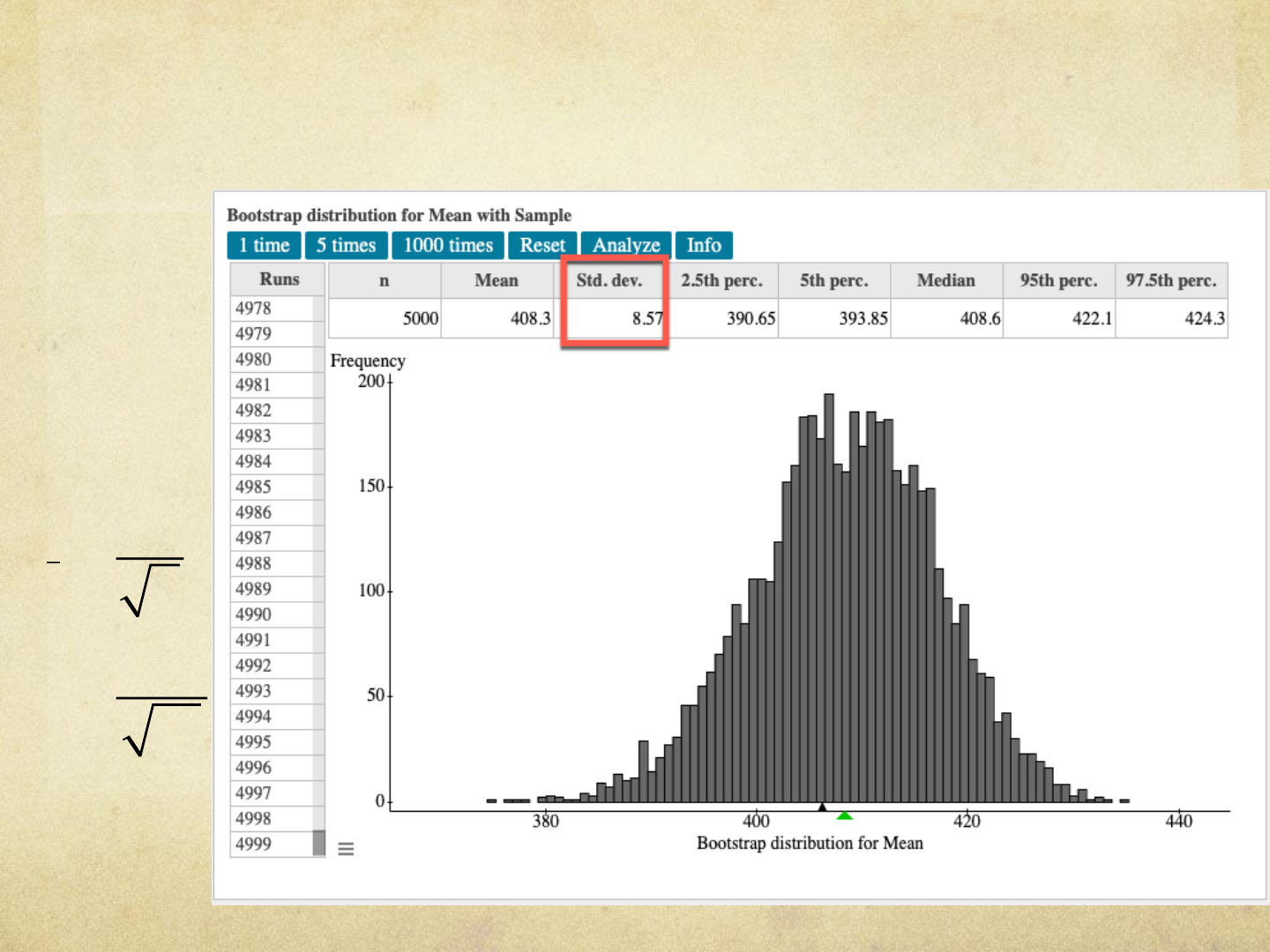
6. Determine the standard deviation of the 5000 bootstrap sample
means. Compare this result to the theoretical standard error of the
sample mean.
25.9
10
8.2
x
n
=
=

7. Construct a 95% confidence interval for the mean distance
of a home run hit in 2021 using Student’s t-distribution.
Compare the result to the bootstrap confidence interval.
Using Student’s t-distribution, we are 95% confident the mean distance of a homerun in
2021 was between 387.2 feet and 429.0 feet. Our bootstrap confidence interval had a
lower bound of 390.7 feet and an upper bound of 424.3 feet.

8. One potential source of variability in estimating the lower and upper bounds of a
bootstrap confidence interval is the randomness around selecting the ten observations
with replacement. Find a second 95% confidence interval for the mean distance of a
homerun using the bootstrap using the same sample data as Part 4. What do you
notice?
We are 95% confident the mean distance of a home run hit in the 2021 season is
between 390.4 feet and 424.5 feet.

9. A second source of variability in estimating the lower and upper bounds of any
confidence interval (bootstrap, or not) is the sample itself.
(a) To illustrate this, obtain a simple random sample of 10 observations from the
population of homerun distances. Write the 10 observations below.
(b) Determine a 95% confidence interval using a bootstrap.
We are 95% confident the mean distance of a homerun is between 374.5 feet and 405.8 feet.

(c) Explain how the two bootstrap intervals differ.

Understanding the Variance Formula:
Why Divide by n – 1?
We are going to work with the HomeRun_2021 data set. This data represents measurements on a variety
of variables for all home runs hit during the 2021 Major League baseball season. This data frame may be
retrieved at either the Interactive Statistics 3/e StatCrunch group or from Github at
https://sullystats.github.io/InteractiveStats3e/Data/HomeRun_2021.csv
To load data into StatCrunch from Github use the following steps.
Step 1: Open StatCrunch.
Step 2: Select Data > Load > From file > on the Web
Step 3: Enter the web address of the data set. Give the data frame of name. Check the box “First line as
column name”. Be sure delimiter is set to comma. Click Upload.
1. The variable “Distance” represents the distance the home run traveled, in feet. Find the
population variance,
, of the distance of all home runs. Note: In StatCrunch, the population
variance is called “Unadj. variance”.
2. The sample variance, s
2
, is computed using the formula
. Why do we divide
by n – 1 instead of n? The reason is that if we divided by n instead of n – 1, the sample variance
would be biased. What does this mean? Essentially, it means that the expected value of the
sample variance would not equal the population variance. Put another way, it means that the
sample variance would consistently over- or under-estimate the population variance. To see how
division by n rather than n – 1 leads to bias, do the following:
(a) Obtain 5000 simple random samples of size n = 9 from the population of all home run
distances. To do this in StatCrunch, select Data > Sample. Choose the variable “Distance”
under Select Columns. Enter 9 in Sample size; enter 5000 in Number of samples. Check the
radio button “Stacked with a sample id”. Check the box “Open in a new data table”. Click
Compute!.
(b) You should now have a new spreadsheet open with a column titled “Sample(Distance)” and a
second column titled “Sample”. Compute the variance of each sample of size n = 9 using the
formula Variance =
. Of course doing this by hand would be miserable, so we are
going to use StatCrunch. Select Stat > Summary Stats > Columns. Under “Select column(s)”
This activity will give you an opportunity to better understand the formula for the sample standard
deviation and why it involves division by n – 1 instead of n. This activity assumes the use of StatCrunch,
however other statistical software may be used instead.

choose “Sample(Distance)”. Under “Group by” choose “Sample” from the drop-down menu.
Under Statistics, choose “Unadj. variance” In StatCrunch, “Unadj. variance” means the
variance is unadjusted for degrees of freedom. This is just a fancy way of saying we are
dividing by n rather than n – 1 in the variance formula. That is, we are computing the
population variance. Finally, select Store in data table. See the figure. Click Compute!
Note: StatCrunch will say “Whoa!! Lots of unique numeric values…”. Simply click Cancel to
avoid binning the data.
(c) In the same spreadsheet, compute the sample variance of each sample of size n = 9 using the
formula
. Again, doing this by hand would be miserable, so we are going to
use StatCrunch. Select Stat > Summary Stats > Columns. Under “Select column(s)” choose
“Sample(Distance)”. Under “Group by” choose “Sample” from the drop-down menu. Under
Statistics, choose “Variance”, which is the sample variance. This is just a fancy way of saying
we are dividing by n rather than n – 1 in the variance formula. Finally, select Store in data
table. See the figure. Click Compute! Note: StatCrunch will say “Whoa!! Lots of unique
numeric values…”. Simply click Cancel to avoid binning the data.
(d) A statistic is said to be biased if its expected value does not equal the value of the parameter.
Expected value is a fancy way of saying the mean. To see whether dividing by n or n – 1
leads to an unbiased estimate of the population variance, compute the mean of the values in
both the “Unadj. variance” column and “Variance” column.
(e) Compare the expected value (mean) of both the “Unadj. variance” and “Variance” values.
Which is closer to the population variance from Part 1? Which formula leads to an unbiased

estimate of the population variance? Explain how dividing by n – 1 helps leads to an
unbiased estimate.
Note: The sample standard deviation,
, is not an unbiased estimate of the
population standard deviation,
. While the explanation as to why this is the case is
beyond the expectations of this course, it has to do with the fact that the square root function is
not a linear function.
